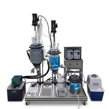
How Do Cstr And Pfr Hydrodynamics Differ From Ideal Models? Real Vs. Simulation

The idealized CSTR and PFR are mathematical fictions—and physical pilot plants prove it every time. In a virtual simulation, a CSTR achieves instantaneous, perfect mixing, while a PFR exhibits a flat velocity profile with zero back-mixing. In a real pilot plant reactor, however, fluid does not read the textbook. Actual hydrodynamics depart from these ideals through axial dispersion, dead zones, channeling, and multiphase slip velocities. These non-idealities directly alter the residence time distribution (RTD) and the measured conversion, making the physical unit a far more complex—and far more instructive—system.

Pilot-scale chemical reactors expose the gap between theory and practice. They seldom display the exponential decay of an ideal CSTR or the sharp residence time delta of a perfect PFR. Instead, they generate skewed RTD curves shaped by incomplete mixing, axial transport, and interfacial mass transfer. The true purpose of a pilot plant is not to replicate an idealization, but to measure these deviations so you can build a validated, non-ideal reactor model.

The Idealized Blueprint: Where Models Assume Perfection

Mathematical simulations start with two extreme, idealized behaviors that make analytical solutions possible. Understanding these baselines is essential before you can appreciate how reality intrudes.

The Perfect Mixer Assumption for CSTR

An ideal Continuous Stirred Tank Reactor assumes the feed is instantly and uniformly distributed throughout the entire volume. Every fluid element has an equal probability of leaving the reactor at any moment, producing a classic exponential RTD. There are no spatial gradients in concentration or temperature.

The Zero Dispersion Plug Flow for PFR

An ideal Plug Flow Reactor assumes fluid moves as a piston with a perfectly flat velocity profile. There is zero mixing in the axial direction and complete mixing in the radial direction. Every fluid element spends exactly the same time inside the reactor, resulting in a sharp impulse RTD and uniform reaction progress along the length.

Hydrodynamic Reality in Pilot Plant Reactors

Physical reactors in teaching and research pilot plants systematically violate every ideal assumption. The fluid mechanics inside are messy, and this messiness is precisely what you need to study.

Axial Dispersion: The Death of the Ideal PFR

In a coiled or tubular pilot plant reactor, the velocity profile is parabolic, not flat. Fluid near the wall moves slower than fluid in the center, causing some molecules to spread out along the flow direction. This axial dispersion smears the residence time distribution. Instead of a sharp spike, you get a broadened peak that reflects the reality of back-mixing and uneven path lengths.

Incomplete Mixing and Dead Zones in Lab CSTRs

A physical continuous stirred tank never achieves perfect homogeneity. Inlet jets can short‑circuit directly to the outlet, while corners or baffled regions form dead zones where fluid stagnates. The result is an RTD curve with a long, decaying tail—fluid elements linger far longer than the ideal mean residence time, skewing conversion predictions downward for slow reactions.

Multiphase Complexities: When Fluids Refuse to Cooperate

Most pilot plants operate with multiple phases. In bubble columns, the gas phase may rise in a plug‑flow‑like manner while the liquid phase remains well‑mixed. In a trickle‑bed or fluidized bed, the solid catalyst, liquid, and gas each have their own residence times and mixing patterns. Slip velocities between phases mean that a single-phase PFR or CSTR model cannot capture the interfacial mass transfer that truly governs reaction rates.

Heat and Mass Transfer Limitations That Shift the Equilibrium

Idealized models often assume isothermal operation and uniform concentration at the catalyst surface. In a pilot plant, spatial temperature gradients and external film resistances are common. In packed‑bed reactors, for instance, heat generation in the center can create a radial temperature profile, while mass diffusion within a catalyst pellet can make the local concentration far different from the bulk fluid. These effects directly cause real product distributions to deviate from the equilibrium curves predicted by pure thermodynamics.

Bridging the Gap: From Ideal Models to Real Performance

The divergence between simulation and pilot plant is not a failure—it is an opportunity. Researchers and students use experimental tools to quantify non‑idealities and then embed them back into mathematical models.

Tracer Studies and Residence Time Distribution (RTD) as a Diagnostic Tool

A stimulus‑response tracer experiment on the pilot plant yields the experimental RTD curve, (E(t)). By comparing the shape of (E(t)) to the ideal exponential or delta function, you can immediately diagnose the character of non‑ideal flow: the size of a dead zone, the intensity of channeling, or the degree of back‑mixing. This single measurement becomes the foundation for all subsequent model adjustments.

Building Compartmental Models to Capture Non‑Idealities

Once the real RTD is known, you can construct a reactor network model—combinations of ideal CSTRs and PFRs in series and parallel—that reproduces the observed curve. For example, a real tubular reactor might be modeled as a plug flow region with a stagnant side‑volume attached. These compartmental models retain the simplicity of ideal equations while accurately reflecting the measured mixing behavior.

The Case of Packed Bed Reactors: Dispersion and Temperature Gradients

In a pilot‑scale packed bed, velocity variations around packing pellets and non‑uniform radial temperature profiles destroy the plug‑flow assumption. To correct for this, researchers superimpose effective transport mechanisms (Fickian diffusion for mass, Fourier conduction for heat) onto the overall plug flow. While this dispersion model becomes a challenging two‑point boundary value problem, it can be approximated by finite‑stage models (treating the bed as interconnected mixing cells) or cross‑flow models that split the void space into stagnant and flowing fractions.

Understanding the Trade‑offs

Pilot plants bring you closer to reality, but they introduce their own interpretive challenges that you must navigate carefully.

Complexity vs. Interpretability: A dispersion model or compartmental network with many adjustable parameters can fit almost any RTD, yet it may hide the true physical mechanism. A model that is “accurate” is not automatically “clarifying.”
Scale‑up Uncertainty: Even when a pilot‑plant model captures hydrodynamics perfectly at the bench scale, the mixing patterns can change dramatically in a full‑sized vessel. RTD data alone may not fully predict industrial behavior without additional scale‑up correlations.
Ignoring Coupled Phenomena: Tracer studies reveal residence time, but they do not directly capture coupled heat transfer or catalyst deactivation. Real performance can drift over hours in a pilot plant while the RTD remains the same, misleading a purely hydrodynamic analysis.
Resource Intensity: Running a physical pilot plant with tracers, analytical instruments, and repeated trials consumes time and materials far beyond a simulation. The educational value is immense, but the cost and complexity are real trade‑offs for a research program.

Making the Right Choice for Your Goal

Your objective determines how deeply you should confront hydrodynamic non‑idealities—and which modeling approach to adopt.

If your primary focus is teaching reactor engineering: Use the pilot plant to visualize the RTD curve. Let students compare the ideal exponential spike with the tailing from a real CSTR, then ask them to explain the discrepancy with dead zones and channeling. This single experiment builds an intuitive, unforgettable link between theory and physical reality.
If your primary focus is research kinetic studies: Prioritize tracer experiments and construct a validated compartmental model for your reactor. Use that calibrated hydraulic model to decouple mixing effects from intrinsic kinetics, so that the rate constants you publish are truly reaction‑limited, not flow‑limited.
If your primary focus is process scale‑up: Combine RTD measurements with temperature profiling and multiphase sampling. A model that captures dispersion in a 2‑liter pilot plant will not necessarily hold in a 2‑cubic‑meter vessel unless you incorporate the dimensionless groups (Reynolds, Bodenstein numbers) that define the mixing regime at both scales.
If your primary focus is bridging simulation and reality for plant operators: Employ the pilot plant as a digital twin validation platform. Force the simulation to match the experimental RTD and temperature profile by adjusting heat transfer coefficients and dispersion lengths, building confidence that the model will predict real‑world excursions.

Only by confronting the fluid’s refusal to behave ideally can you truly master the scale‑up, optimization, and safe operation of real chemical processes.

Summary Table:

Reactor Type	Ideal Model Assumption	Physical Pilot Plant Reality	Key Hydrodynamic Deviations
CSTR	Instantaneous, perfect mixing; no spatial gradients.	Short-circuiting, bypassed zones, and stagnant regions.	Dead zones, bypass flow, skewed RTD tail
PFR	Flat velocity profile; zero axial mixing; uniform RTD.	Parabolic velocity profile; molecules travel at different speeds.	Axial dispersion, back-mixing, broadened RTD
Multiphase	Single-phase continuous flow; constant velocity.	Multiple phases travel at different velocities; mass transfer limits.	Slip velocities, radial temperature gradients

Bring Real-World Reactor Hydrodynamics to Your Lab

Teaching reactor design requires physical systems that expose the limits of ideal simulations. LABPARK provides state-of-the-art Educational and Vocational Unit Operations Pilot Plants in chemical engineering, bioprocess & biotech, and environmental & water treatment.

Specifically designed for universities, research institutes, and enterprises, our pilot plants enable students and researchers to perform precise tracer studies, analyze RTD curves, and model real-world non-idealities.

Ready to upgrade your lab's hands-on training capabilities? Contact LABPARK today to discuss your custom pilot plant needs!