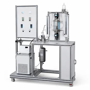
How To Determine Overall Heat Transfer Coefficient (K) In Unit Operations Pilot Plants With Variable Fluid Properties

Variable fluid properties break the standard assumption of a constant K—but researchers can still obtain accurate values by matching the calculation method to the temperature-dependence of the coefficient. In unit operations pilot plants, when fluid temperatures shift dramatically, the overall heat transfer coefficient (K) changes because viscosity, thermal conductivity, and density all vary with temperature. The surface-level answer is that you must either apply a modified log-mean-temperature-difference equation if K varies linearly with temperature, or divide the exchanger into smaller segments and treat K as constant within each when the variation is non-linear. Both approaches transform a seemingly intractable problem into a manageable, step‑wise calculation grounded in fundamental heat transfer principles.

The central insight is that no single formula applies to all temperature ranges. The choice between a modified analytical equation for a linearly varying K and a numerical segmentation for non-linear K directly determines the accuracy of your area calculation and the validity of your pilot‑plant data. Get the method right, and you turn problematic property changes into a precise research tool rather than a source of error.

The Core Challenge: Variable Properties

When fluid temperatures change by 50°C or more in a single pass, the physical properties that define the film coefficients on each side of the heat transfer surface do not stay constant. This directly alters the local K value along the heat exchanger length.

Why Fluid Properties Change with Temperature

Viscosity often drops sharply as temperature rises, while thermal conductivity may increase or decrease depending on the fluid. For liquids, a temperature rise typically lowers viscosity, improving turbulence and raising the convective coefficient on that side. Gases can show the opposite trend. These shifts mean the overall resistance to heat flow is a moving target.

The Consequence for the Overall Heat Transfer Coefficient

Assuming a single, constant K when properties vary leads to significant errors in the calculated heat transfer area. The standard equation $Q = K A \Delta T_m$ depends on a representative, averaged $\Delta T_m$ and a single K—but if K itself is a function of temperature, that average no longer captures the physics. The pilot plant designer must instead account for the temperature-dependent K profile.

Method 1: When K Varies Linearly with Temperature

If experimental data or first-principles estimates show that K changes in direct proportion to the fluid temperature difference, a clean analytical solution exists.

The Modified Heat Rate Equation

The approach replaces the standard log mean temperature difference with a modified form that uses the local K values at both ends of the exchanger. The equation from the primary reference is:

$Q = S_o \cdot \frac{K_{o1} \Delta t_2 - K_{o2} \Delta t_1}{\ln\left(\frac{K_{o1} \Delta t_2}{K_{o2} \Delta t_1}\right)}$

Here, $K_{o1}$ and $K_{o2}$ are the local overall heat transfer coefficients evaluated at the hot end and cold end, respectively. $\Delta t_1$ and $\Delta t_2$ are the corresponding local temperature driving forces.

Interpreting the Local Coefficients

$K_{o1}$ and $K_{o2}$ are not measured directly; they are computed from the convective film coefficients, wall conduction, and fouling resistances at each terminal temperature. This requires evaluating all fluid properties at the inlet and outlet temperatures, a task that fits naturally into a pilot plant’s educational framework because students must gather property data and compute resistances point by point.

Practical Implementation in Pilot Plants

For a counter-current or co-current flow arrangement, you first measure steady‑state inlet and outlet temperatures. You then determine $K_{o1}$ and $K_{o2}$ using standard resistance-in-series models ($1/K = 1/h_o + 1/h_{od} + \dots$) at each terminal condition. Plugging these into the modified equation yields the correct heat duty-to-area relationship without needing to segment the exchanger.

Method 2: Handling Non-Linear Variation of K

What if K does not follow a simple straight line with temperature? Many real systems—especially those involving phase change, highly viscous oils, or large property gradients—exhibit curved, non‑linear K‑temperature profiles.

The Segmentation Approach

The most intuitive strategy is to divide the heat exchanger into a series of small, virtual segments. Within each segment, the temperature change is small enough that K can be treated as constant. The LMTD method is then applied segment by segment, and the total area is the sum of the segment areas.

Numerical and Graphical Integration

For a rigorous solution, the differential heat rate equation $dQ = K(T) , \Delta T , dS$ is integrated numerically. Researchers plot or tabulate the function $1/(K \Delta T)$ against the cumulative heat duty $Q$, and the area is found from the area under the curve. Today, spreadsheet‑based trapezoidal or Simpson’s rule integrations are standard in student labs, replacing the old graphical methods but still teaching the same principle.

Selecting the Proper Qualitative Temperature for Dimensionless Numbers

An often‑overlooked step is choosing the reference temperature at which to evaluate physical properties when calculating $K$. For low‑viscosity fluids in forced convection, the arithmetic mean of inlet and outlet temperatures works well as the qualitative (bulk) temperature. For high‑viscosity liquids where the Sieder‑Tate correction applies, all properties except the wall‑adjacent viscosity are evaluated at the bulk temperature; the wall viscosity demands the average tube‑wall temperature. Getting this choice wrong distorts the predicted K variation and undermines the segmentation.

Experimental Determination as a Foundational Step

Before deciding between the linear and non-linear methods, students must often measure K experimentally under representative conditions to understand the nature of the variation.

Steady-State Heat Balance and LMTD Method

In a pilot‑scale shell‑and‑tube or plate exchanger, students operate at steady state, measure all inlet/outlet temperatures and flow rates, calculate the heat load $Q = \dot W c_p \Delta T$, and then solve $K = Q / (A , \Delta T_m)$ using the log mean temperature difference. Repeating this at several average temperature levels—while keeping the same fluids and flow rates—reveals whether K changes linearly or non‑linearly as the temperature span shifts.

Wilson Plot for Reactor Jackets

For jacketed reactors used in unit operations training, the Wilson plot is a powerful tool. By measuring K at several agitator speeds and plotting $1/K$ against $n^{-2/3}$, the y‑intercept gives the maximum achievable $K_{max}$ free from wall effects. This method is independent of the solvent and provides a clean reference point, helping students decouple film resistances from the overall coefficient when properties vary.

Role of Empirical Ranges for Validation

Published ranges—such as 850–1700 W/(m²·°C) for water‑to‑water or 17–280 W/(m²·°C) for water‑to‑gas— serve as sanity checks. If a calculated segment K falls far outside the expected bracket for the given fluid combination, it signals a measurement or property‑evaluation error, or that the assumption of linearity might be invalid.

Understanding the Trade‑offs and Common Pitfalls

Every method for handling variable K comes with its own set of compromises. Being aware of them prevents misapplication and builds critical thinking.

Accuracy vs. Complexity

The linear modified equation is computationally light and ideal for a classroom demonstration, but it fails if the K‑temperature relationship is even slightly curved. Segmentation and numerical integration provide near‑exact results but demand more measurement points and careful data reduction—time that may be scarce in a short lab session.

Pitfalls in Selecting the Qualitative Temperature

Using the wrong bulk temperature to evaluate properties feeds errors directly into K. For example, employing the inlet‑outlet arithmetic mean for a high‑viscosity oil that displays a 100 °C temperature drop can underestimate the film coefficient because the mean viscosity is much higher than the local value near the hot end. The result is a distorted K profile that leads to wrong conclusions about linearity.

Limitations of Empirical Correlations

Empirical equations for film coefficients (e.g., Dittus‑Boelter, Sieder‑Tate) have their own valid ranges for Reynolds and Prandtl numbers. When large temperature swings cause the flow regime to transition from turbulent to transitional, the correlation may no longer be accurate. This introduces error into the predicted local K values, regardless of the integration method.

The Risk of Extrapolating Point Measurements

Measuring K at only two operating points and fitting a straight line can mask a non‑linear trend. In pilot‑plant research, always gather at least three or four data points at different temperature spans to verify linearity before applying the simplified modified equation.

Making the Right Choice for Your Pilot‑Plant Study

The optimal approach depends on your learning objective, the fluids involved, and the accuracy you need.

If your primary focus is an educational demonstration of temperature‑dependent properties: Use the modified linear equation on a system that genuinely shows linear K variation (e.g., moderate‑temperature water‑water exchange) to teach the concept without overwhelming students with numerics.
If your primary focus is high‑accuracy design data for scale‑up: Employ the segmentation method or numerical integration, and back up the results with at least three experimental K values at different temperature levels to map the true variation.
If your primary focus is handling a high‑viscosity or phase‑change fluid: Always default to the segmentation approach, evaluate all properties at the correct qualitative temperature, and use the Wilson plot to separate wall and film resistances when possible.
If your primary focus is a quick verification of a pilot‑plant performance: Compute K from a single steady‑state run using the LMTD method, but treat the result as an average coefficient valid only at that exact temperature span. Never use it to predict performance at a dramatically different span without checking for variation.

Understanding how to determine K when fluid properties change is not a single recipe—it is a disciplined framework that connects thermodynamics, transport phenomena, and experimental technique. Choose the method that matches the physics of your system, and your pilot‑plant data will serve you reliably from the teaching lab to the design office.

Summary Table:

Method	Fluid K Behavior	Calculation Approach	Best Application
Linear Method	Proportional to temp difference	Modified LMTD with terminal K values	Simple fluids, moderate temp spans
Segmentation	Curved/Non-linear profile	Multi-segment LMTD & numerical integration	Viscous fluids, phase changes, large spans

Optimize Your Chemical Engineering Labs with LABPARK

Accurate heat transfer analysis requires reliable, high-precision equipment. LABPARK provides premium Educational and Vocational Unit Operations Pilot Plants in chemical engineering, bioprocess & biotech, and environmental & water treatment. Designed specifically for universities, research institutes, and enterprises, our pilot plants empower students and researchers to master complex calculations like variable heat transfer coefficients with real-world accuracy.

Ready to upgrade your laboratory capabilities? Contact LABPARK today to request a quote or discuss your custom pilot plant requirements!