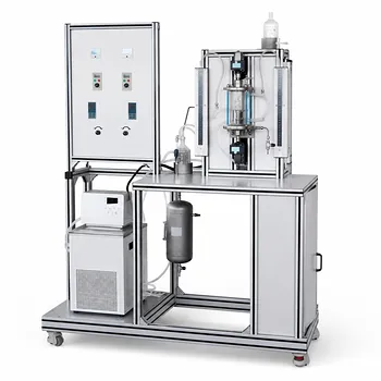
How To Determine Maximum Heat Transfer Coefficient In Reactor Pilot Plants: Wilson Plot Guide

The Wilson plot method is the most reliable experimental technique for determining the maximum overall heat transfer coefficient ((U_{max})) in a stirred reactor. By measuring the overall heat transfer coefficient at several stirrer speeds and extrapolating the data, the resistance from the process-side fluid film is eliminated, revealing the intrinsic heat transfer capability of the unit.

The core insight: Plotting (1/U) versus (n^{-2/3}) from cooling curves taken at different stirring speeds yields a straight line whose y-intercept gives (1/U_{max}). This value is independent of the solvent and represents the ceiling of heat transfer performance when agitation is no longer the limiting factor.

Why (U_{max}) Matters in Reactor Pilot Plants

The Heat Transfer Bottleneck

In a jacketed reactor, the overall heat transfer coefficient (U) is a combination of the jacket-side film coefficient, the wall resistance, and the vessel-side film coefficient. For many liquid-phase reactions, the vessel-side film resistance dominates. As stirring speed increases, the vessel-side coefficient improves, and (U) climbs toward an asymptote—this is (U_{max}).

A Scale‑Up Imperative

Knowing (U_{max}) tells engineers the absolute best heat removal capacity of the reactor geometry. Because heat transfer area scales with (V^{2/3}) while heat generation scales with (V), this ceiling becomes critical when assessing if a pilot reactor can safely handle an exothermic reaction at production scale.

The Wilson Plot Method: Step by Step

1. Run Cooling Curves at Multiple Stirrer Speeds

Fill the reactor with a chosen solvent to the intended process volume. Set the jacket to a constant heating (or cooling) temperature and allow the batch to reach a steady elevated temperature. Then, switch to a cooling mode and record the batch temperature over time at a fixed, well-defined stirrer speed.

Repeat the cooling curve for at least four other stirrer speeds, covering the full practical range of the agitator.

2. Calculate (U) for Each Speed

From each cooling curve, use the transient heat balance:

[ m c_p \frac{dT}{dt} = U A (T_{jacket} - T) ]

By fitting the temperature-time data, the lumped parameter (UA)—and thus (U) if the wetted area (A) is known—is extracted for that stirring speed. Consistent jacket temperature control and accurate temperature logging are essential.

3. Construct the Wilson Plot

Create a graph with the reciprocal of the overall heat transfer coefficient on the y‑axis and the stirrer speed raised to the (-2/3) power on the x‑axis. The theoretical basis rests on the fact that turbulent heat transfer in stirred vessels scales with (Re^{2/3}), so the vessel-side film resistance is proportional to (n^{-2/3}).

The data will form a straight line:

[ \frac{1}{U} = \frac{1}{U_{max}} + b \cdot n^{-2/3} ]

4. Extract (U_{max})

The y-intercept of the best-fit line is exactly (1/U_{max}). Because the intercept represents the sum of the constant thermal resistances (jacket film, wall, and any systematic offset), this value is the ceiling (U) that cannot be surpassed by more vigorous stirring.

Why This Works (and Why the Solvent Choice Doesn’t Matter)

The Self‑Cancelling Extrapolation

The Wilson plot isolates the variable resistance (vessel-side film) from all other resistances that are independent of stirrer speed. As long as the vessel-side film coefficient follows a power‑law relationship with (n), the linearization holds. The method is famously independent of the solvent because any error in solvent properties shifts the data points proportionally but does not change the intercept.

Solvent Recommendations

While any stable liquid can be used, isopropanol is highly suitable for educational and pilot reactors. Its moderate viscosity and well-characterized thermal properties yield clean, linear Wilson plots without the hazards or cleaning issues of more exotic fluids.

A Quick Estimation Method

The Single‑Point Approximation

For a rapid, albeit approximate, determination of (U_{max}), fill the reactor with water and stir at the maximum possible speed. Under these conditions, the vessel-side film resistance is minimized, and the measured (U) will be a close approximation of the true (U_{max}). This shortcut is useful for quick screening or when time constraints prevent a full Wilson plot study.

Understanding the Trade-offs

Accuracy vs. Experimental Effort

The Wilson plot requires multiple careful cooling experiments and precise curve fitting, which consumes significant lab time and solvent. The quick method offers less precision but can be completed in a single run. Students must weigh the depth of insight against available resources.

Assumptions and Limitations

Power‑law exponent. The (-2/3) scaling applies to fully turbulent flow in standard baffled vessels. Atypical geometries or very low stirring speeds may deviate from this rule.
Constant jacket-side coefficient. The method assumes the jacket-side resistance remains unchanged across the speed range; a tightly controlled jacket utility is necessary.
No fouling or phase change. The analysis presumes clean heat transfer surfaces and no boiling or condensation that would alter the film coefficients in non‑linear ways.

Educational Value

From a teaching perspective, the Wilson plot elegantly combines hands‑on plant operation, data fitting, and the conceptual separation of thermal resistances. It transforms an abstract textbook coefficient into a tangible, measurable limit.

Making the Right Choice for Your Goal

The appropriate approach depends entirely on what you need the (U_{max}) value for.

If your primary focus is a rigorous research-grade characterization: Perform the full Wilson plot with isopropanol, using at least five stirrer speeds. This yields the most reliable, solvent-independent (U_{max}) that can be carried into scale‑up calculations.
If your primary focus is rapid screening for a potential reaction: Use the quick water‑test at maximum stirring to obtain an approximate (U_{max}) in a single experiment. It’s enough to make go/no‑go decisions on thermal safety.
If your primary focus is student learning and demonstration: Walk through the entire Wilson plot procedure, but let students compare the quick approximation to the extrapolated value. This teaches both the theory and the pragmatic trade‑offs of experimental heat transfer.

A well-characterized (U_{max}) turns a pilot reactor into a predictive tool, giving students and researchers the confidence to scale chemistry safely and efficiently.

Summary Table:

Method	Accuracy	Experimental Effort	Main Advantage	Best Suited For
Wilson Plot Method	High (Extrapolated)	High (Requires multiple cooling runs)	Solvent-independent & highly rigorous	Academic Research & Scale-up
Single-Point Approximation	Moderate / Low	Low (Single high-speed water run)	Fast, simple setup	Quick Screening & Demos

Bring Hands-On Reactor Engineering to Your Lab

Looking to equip your facility with state-of-the-art pilot plants? LABPARK provides premium Educational and Vocational Unit Operations Pilot Plants in chemical engineering, bioprocess & biotech, and environmental & water treatment.

Designed specifically for universities, research institutes, and enterprises, our advanced training systems make complex thermodynamic concepts like the Wilson plot method easy to demonstrate, visualize, and calculate.

Contact LABPARK today to discuss your laboratory requirements and get a customized solution!