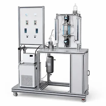
How To Differentiate Equimolar Counterdiffusion And Stagnant Gas Diffusion? Pilot Plant Guide

In mass transfer education, the leap from textbook equations to real-world pilot plants hinges on seeing the boundary condition—whether the net molar flux of the inert gas is zero or balanced—come to life. Instructors differentiate equimolar counterdiffusion from diffusion through a stagnant gas by using pilot plants where the bulk flow of the inert carrier can be either purposely balanced (as in a diffusion coefficient measurement cell) or deliberately stagnated (as in a gas absorption column). The setup immediately reveals whether the drift factor—the convective contribution to molar flux—must be applied, cementing the link between process type, flux equation, and industrial unit operation.

The critical distinction lies in the boundary condition for the inert component: equimolar counterdiffusion forces its flux to balance the diffusing species, eliminating bulk flow, while stagnant‑gas diffusion sets its flux to zero, creating a convective drift that accelerates mass transfer. Pilot plants make this tangible by controlling whether an inert gas is moving or not.

The Two Diffusion Regimes: A Boundary Condition Problem

Both mechanisms describe how a species moves through a gas mixture, but their mathematical forms diverge because of what happens to the other component.

Equimolar Counterdiffusion: Zero Net Molar Flux

In equimolar counterdiffusion, the molar fluxes of the two species are equal in magnitude and opposite in direction.
This means the net total molar flux is zero—no bulk flow develops.
Distillation columns are classic examples, where the vaporization of a volatile component is perfectly balanced by the condensation of a less volatile one.

Diffusion Through a Stagnant Gas: Flux of the Inert Is Zero

Here, the carrier gas is stagnant—its molar flux is zero.
As the diffusing species moves through the stationary inert, a convective drift arises to maintain zero net velocity of the inert.
This is the norm in gas absorption and desorption pilot plants, where a solute gas transfers through a static gas film into a liquid solvent.

Turning Concepts into Practice: Pilot Plant Demonstrations

The power of pilot plants lies in making these boundary conditions physically observable, forcing students to choose the correct flux equation.

The Gaseous Diffusion Cell for Equimolar Counterdiffusion

A dedicated gaseous diffusion pilot plant directly validates Fick’s law for equimolar counterdiffusion.
The apparatus maintains a constant partial pressure difference of the diffusing species across a tube of known length and temperature.
Because both ends of the tube allow the inert gas to move freely, no bulk flow builds up—the fluxes balance.

Students measure the steady‑state molar flux ( N_A ) and directly apply the simplified integrated flux equation:
( N_A = \frac{D \cdot (p_{A1} – p_{A2})}{R \cdot T \cdot z} )
This method yields the experimental diffusion coefficient without any drift‑factor correction. Precise temperature control and stable gas flow management ensure the steady‑state assumption holds, reinforcing the link between a zero‑net‑flux condition and the simplest form of Fick’s law.

The Absorption Column for Stagnant Gas Diffusion

In a gas absorption pilot plant (e.g., a packed column with a falling liquid film), the inert carrier gas is stationary relative to the diffusing solute.
Students observe that the solute’s flux is larger than predicted by pure molecular diffusion alone because a bulk flow develops to push the solute through the stagnant layer.
Instructors then introduce the drift factor ( (1 + y_A) ) in the flux equation:

[ N_A = \frac{D}{R T z} \cdot \frac{P}{p_{B,lm}} \cdot (p_{A1} – p_{A2}) ]

where ( p_{B,lm} ) is the log‑mean partial pressure of the stagnant inert.
The need for this correction becomes a memorable lesson—the pilot plant’s measured outlet concentration simply cannot be matched without it, dramatically illustrating the impact of a non‑zero convective term.

Understanding the Trade-offs

Pilot‑plant demonstrations make concepts stick, but they also expose where students commonly misapply models.

Accuracy vs. Conceptual Overload

The drift factor is essential for designing absorbers, yet it adds algebraic complexity.
If students are not fully comfortable with log‑mean driving forces, they may misinterpret the correction as an empirical fix rather than a physical consequence of a stagnant inert.
Instructors must balance the depth of mathematical derivation with the clarity of the physical picture.

Steady-State Assumptions and Real Control

Both demonstrations rely on a steady‑state concentration profile.
Any fluctuation in temperature, flow rates, or liquid‑phase concentration in the absorption column can corrupt the computed flux.
High‑quality pilot plants compensate with precise instrumentation, but students must learn to judge when the assumption truly holds.

Making the Right Choice for Your Teaching Lab

The selection of pilot‑plant demonstrations should align with the core learning objective.

If your primary focus is teaching Fick’s law fundamentals: Use the gaseous diffusion cell—it isolates equimolar counterdiffusion, yielding a clean, direct measurement of the diffusion coefficient without the drift factor.
If your primary focus is industrial absorber or stripper design: Deploy the absorption column to show how a stagnant inert introduces a convective term that cannot be ignored in real‑world flux calculations.
If your primary focus is comparing process types side‑by‑side: Run both experiments sequentially so students can contrast the zero‑net‑flux condition with the stagnant‑inert condition and immediately see when the drift factor is required.

By grounding the distinction in their own pilot‑plant data, instructors transform an abstract boundary condition into an unforgettable engineering insight.

Summary Table:

Feature	Equimolar Counterdiffusion	Diffusion Through Stagnant Gas
Net Molar Flux	Zero ($N_A = -N_B$)	Non-zero ($N_B = 0$)
Convective Drift	None (No drift factor needed)	Present (Requires drift factor correction)
Pilot Plant Setup	Gaseous Diffusion Cell	Gas Absorption Column
Industrial Application	Distillation columns	Gas absorption/desorption

Elevate Your Engineering Lab with LABPARK

Bridging the gap between theoretical mass transfer equations and physical reality requires robust, precisely controlled equipment. LABPARK provides premium Educational and Vocational Unit Operations Pilot Plants in chemical engineering, bioprocess & biotech, and environmental & water treatment for universities, research institutes, and enterprises.

Our pilot plants—including advanced gas absorption columns and diffusion cells—are engineered to help your students and researchers easily visualize boundary conditions, master flux equations, and gain hands-on industrial experience.

Ready to upgrade your laboratory instrumentation? Contact LABPARK today to request a catalog or discuss your custom lab requirements with our specialists!