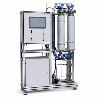
How Does Hopf Bifurcation Modeling Apply To Cstr Pilot Plants? Theory Vs. Practical Operation

The Hopf bifurcation point is not just an abstract mathematical concept—it is a physical threshold you can observe, manipulate, and verify on a CSTR pilot plant. Mathematical models based on nonlinear ordinary differential equations (ODEs) predict where a reactor will spontaneously transition from a stable, steady-state operation to self-sustained temperature and concentration oscillations. A unit operations training system turns these predictions into hands-on reality: by adjusting parameters like the Damköhler number or heat transfer coefficient, you can induce the very instability the equations describe, observe the resulting oscillatory behavior, and directly connect the theory of stability analysis (including Floquet multipliers) to critical process control skills.

While Hopf bifurcation theory provides the analytical map of stability boundaries, a CSTR training system serves as the physical ground truth—showing not only when oscillations begin, but also how real-world imperfections like heat loss or sensor lag alter the predicted behavior. This closes the gap between mathematical modeling and practical, safe reactor operation.

The Mathematical Roots: Stability and Oscillation

How Nonlinear ODEs Define Reactor Behavior

A CSTR’s dynamics are governed by mass and energy conservation equations that describe concentration and temperature changes over time. These equations form a system of nonlinear ordinary differential equations (ODEs) that can exhibit multiple steady states.

The nonlinearity comes from the reaction rate term, often following Arrhenius kinetics. This creates conditions where small changes in inputs can lead to large, qualitative changes in the system’s trajectory.

The Hopf Bifurcation as a Stability Switch

A Hopf bifurcation occurs when a pair of complex conjugate eigenvalues of the linearized system crosses the imaginary axis. Mathematically, this marks the point where a steady state loses stability and gives birth to a limit cycle—a periodic orbit.

Beyond this critical point, the reactor no longer settles to a constant temperature and conversion. Instead, it cycles continuously, with the amplitude of oscillation determined by the nonlinear terms.

The Role of Floquet Multipliers

Once a limit cycle exists, its stability is assessed using Floquet theory. Floquet multipliers indicate whether the periodic orbit is stable or unstable. A stable limit cycle corresponds to the sustained, repeatable oscillations you can actually observe in a real reactor.

From Equations to Pilot Plant: Verifying Bifurcation Points

Damköhler Number as Your Primary Control Knob

In a CSTR training system, the Damköhler number (Da)—the ratio of reaction rate to convective transport rate—becomes a tangible lever. You manipulate Da by varying the feed flow rate or the reactant concentration.

Operating the pilot plant at a series of increasing Da values will first show steady-state conversion. At a critical Da predicted by the model, the reactor’s temperature and outlet conversion will begin to oscillate spontaneously, sometimes after a tiny perturbation. This is the physical manifestation of the Hopf bifurcation.

Heat Transfer Conditions and the Path to Instability

Many exothermic CSTR reactions exhibit Hopf bifurcations when the heat transfer capacity is reduced. On a training system, you might lower the coolant flow rate or raise the jacket setpoint temperature to cross the stability boundary.

The physical feedback loop is clear: a slight temperature increase accelerates the reaction, which generates more heat. If cooling cannot remove it fast enough, the temperature rises further, then reactant depletion slows the reaction, the temperature drops, and the cycle repeats—exactly as the model predicts.

Seeing the Unseen: Observing Physical Indicators of Bifurcation

Oscillation Onset and Amplitude Growth

As you approach the bifurcation point, the reactor’s response to a small step disturbance changes dramatically. Instead of a smooth return to a steady state, the temperature overshoots and takes longer to settle, a phenomenon called critical slowing down.

Past the bifurcation, any tiny fluctuation triggers sustained oscillations. The amplitude starts small near the bifurcation point (a supercritical Hopf) and grows as you move further into the unstable region, or it may jump abruptly (a subcritical Hopf), revealing the nature of the nonlinearity.

Hysteresis and the Unstable Branch

A crucial practical lesson is that the bifurcation can exhibit hysteresis. By reversing the path—slowly increasing the Damköhler number until oscillations appear, then decreasing it—you might find that the oscillations persist beyond the onset point. This reveals the presence of an unstable periodic branch that the model predicts but cannot be observed directly; the training system lets you infer its existence from the hysteretic loop.

Understanding the Trade-offs

Ideal Models vs. Imperfect Reality

Mathematical models assume perfect mixing, known kinetics, and no heat loss. Your pilot plant has mixing inefficiencies, wall heat losses, and sensor lags. These real-world deviations can shift the exact location of the bifurcation point or round off the sharp transition.

This discrepancy is not a failure; it’s the primary educational value. You learn to interpret why the model predicts a bifurcation at Da=1.2 but the reactor oscillates at Da=1.5, and you develop the diagnostic skills to identify which real-world effect is responsible.

The Pitfalls of a Purely Theoretical Approach

Relying solely on the mathematical model can be misleading. A predicted stable steady state might be operationally unattainable because of an overlooked imperfection, or a predicted unstable region might be manageable in practice with active control.

Conversely, over-focusing on the pilot plant without the model leaves you blind to the underlying structure. The bifurcation analysis tells you where to look and what the potential dynamic regimes are, saving hours of aimless experimentation.

Safety and Process Control Implications

From a practical standpoint, an unforeseen Hopf bifurcation in a production reactor can be disastrous, leading to thermal runaway or off-spec product. Training on a pilot plant teaches you to recognize the pre-bifurcation signatures—such as increased sensitivity to perturbations—and to engineer a safe margin from the stability boundary.

Making the Right Choice for Your Goal

How you use the CSTR training system with respect to Hopf bifurcation depends on your primary objective.

If your primary focus is mastering nonlinear dynamics theory: Use the pilot plant to verify the model’s predictions systematically. Vary the Damköhler number in small increments near the predicted bifurcation point, record the oscillation amplitude and frequency, and compare them to the Floquet analysis. The goal is to see the abstract become concrete.
If your primary focus is developing practical process control skills: Deliberately operate the reactor across the stability boundary to learn how to detect the onset of oscillation and how to bring the reactor back to a safe steady state using temperature or feed control loops. The focus is on intervention, not just observation.
If your primary focus is troubleshooting real-world reactors: Use the training system to explore deviations from ideality—intentionally introduce a heat loss or a mixing defect, and map how the bifurcation point shifts. This builds a mental library of non-ideal behaviors that purely mathematical study cannot provide.

The mathematical modeling of Hopf bifurcations transforms from an exercise in eigenvalue analysis into a physical diagnostic tool the moment you stand before a CSTR training system and watch the temperature needle begin to cycle, knowing exactly which equation predicted that very swing.

Summary Table:

Aspect	Mathematical Model (Theory)	CSTR Pilot Plant (Reality)
Core Dynamics	Predicts stability & limit cycles using nonlinear ODEs	Observes physical temperature & concentration oscillations
Control Variables	Manipulates Damköhler number (Da) analytically	Adjusts flow rates, feed concentrations, & jacket cooling
System Conditions	Assumes perfect mixing, no heat loss, & zero sensor lag	Features real-world heat loss, mixing defects, & sensor lag
Stability Diagnostics	Analyzes Floquet multipliers and eigenvalues	Observes critical slowing down, hysteresis, & amplitude growth

Bring Complex Reactor Dynamics to Life with LABPARK

Bridging mathematical theory and hands-on operational expertise is critical for training tomorrow's engineers. LABPARK provides premium Educational and Vocational Unit Operations Pilot Plants in chemical engineering, bioprocess & biotech, and environmental & water treatment.

Specifically designed for universities, research institutes, and enterprises, our training systems enable students and operators to safely visualize complex reactor phenomena, manage process instabilities, and master real-world control loops.

Ready to elevate your engineering lab? Contact our specialists today to find the ideal pilot plant configuration for your training goals.