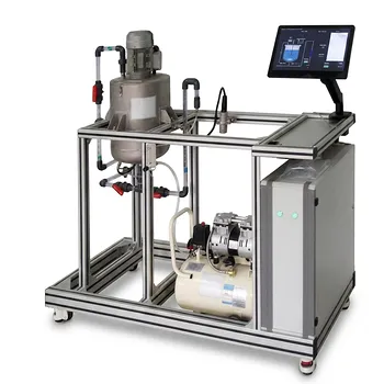
How Do Educational Pilot Plants Help Visualize Reynolds Numbers? Master Laminar & Turbulent Flow.

A dye filament in a glass pipe bridges the gap between abstract equations and physical reality.

Vocational and educational pilot plants make the Reynolds number (Re) tangible by using clear test sections and a dye injection system to visualize flow regimes. Students adjust a control valve, measure volumetric flow rate, calculate fluid velocity, and compute Re. They then watch the dye streak transition from a stable thin line (laminar) to chaotic dispersion (turbulent), directly correlating the dimensionless number with observed pipe flow behavior.

The core insight: These pilot plants transform the Reynolds number from a textbook formula into a visceral learning experience. Students not only calculate Re but simultaneously witness the precise thresholds—laminar below 2000, transitional up to 4000, and turbulent beyond—that govern all pipe flow. This dual feedback loop of measurement and immediate visual feedback cements an intuitive, lasting understanding of fluid dynamics.

The Experimental Setup: Visualizing the Invisible

A well-designed pilot plant strips away complexity so the underlying physics becomes unmistakable. The system’s transparency and instrumentation enable students to see and quantify what is normally hidden inside industrial pipelines.

The Core Components of a Flow Visualization Pilot Plant

The heart of the system is a clear acrylic or glass pipe mounted horizontally or vertically. A fine dye injector places a stream of colored liquid (often ink or potassium permanganate) precisely at the pipe centerline. A flow control valve downstream lets the operator smoothly vary the flow rate, while a flow meter or a timed collection vessel yields the volumetric flow. A thermometer or thermocouple records the water temperature, which is essential for determining viscosity and density.

The Power of Dye Injection in a Transparent Section

Dye injection turns abstract flow patterns into a visible narrative. At low velocities, the dye remains a sharp, thread-like filament that glides down the pipe without mixing. As the flow increases, the filament begins to waver, break into eddies, and finally disperse rapidly throughout the cross-section. This real‑time visual cue immediately signals which regime the fluid occupies, long before any calculation is complete.

Calculating the Reynolds Number from Raw Data

The pilot plant provides the few variables needed to compute Re, teaching students how this dimensionless group arises from basic measurements.

From Volumetric Flow Rate to Average Velocity

Students first determine the average flow velocity ((u)). Using the measured volumetric flow rate ((Q)) and the known cross‑sectional area of the pipe ((A = \pi D^2/4)), they calculate (u = Q/A). This simple step illustrates that the average velocity is not a direct reading but a derived quantity, linking the pump setting to a key fluid property.

Accounting for Fluid Properties via Temperature

The density ((\rho)) and dynamic viscosity ((\mu)) of water change significantly with temperature. By measuring the water temperature and consulting standard tables, students find the correct values. The Reynolds number is then calculated as:

[ Re = \frac{\rho , u , D}{\mu} = \frac{u , D}{\nu} ]

where (\nu) is the kinematic viscosity. This process reinforces that Re is not merely a number but a ratio of inertial forces to viscous forces, directly influenced by real‑world conditions.

Computing Re and Predicting the Regime

With the calculation complete, students can predict the flow regime based on well‑established thresholds:

Laminar flow: (Re \le 2000)
Transitional flow: (2000 < Re < 4000)
Turbulent flow: (Re \ge 4000)

The pilot plant then allows immediate comparison between this numerical prediction and what the dye actually does.

Bridging Theory and Observation: Correlating Re with Flow Patterns

The real educational power emerges when the calculated Re is matched against the visible dye behavior, creating a mental model that lasts.

Laminar Flow (Re < 2000): The Delicate Filament

At low Re, viscous forces dominate. The dye forms a clean, straight, parallel line that stays intact along the pipe. Any small disturbance damps out quickly, and the flow appears perfectly orderly. Students can see that the fluid particles move in layers with no macroscopic mixing, exactly as the theory describes.

Transitional Flow (2000 < Re < 4000): The Wavering Streak

As the valve is opened further, the dye streak begins to oscillate, flicker, or break intermittently. This visually marks the boundary where inertia starts to overwhelm viscosity. The flow may shift between laminar-like and turbulent-like bursts, vividly demonstrating why this range is called the transition zone and why it is sensitive to external vibrations or inlet disturbances.

Turbulent Flow (Re > 4000): Rapid Dispersion

Beyond the critical Re, inertia completely dominates. The dye flashes into a cloud almost immediately after injection, spreading across the entire pipe cross-section. The chaotic, eddying motion is impossible to miss. This visual starkly contrasts with the laminar filament and solidifies the concept that turbulent flow dramatically enhances mixing and momentum transfer.

Beyond the Visual: Connecting Re to Engineering Parameters

Pilot plants often include additional measurement points to show that Re is not an academic curiosity but the key to predicting real system behavior.

Demonstrating the Entry Length to Develop Flow

Some pilot plants have a long transparent section that reveals the hydrodynamic entrance region. For laminar flow, the entry length ((x_0)) needed for the velocity profile to become fully developed follows (x_0/D = 0.057 , Re). By adjusting the flow rate while keeping the flow laminar, students can visually observe how a higher Re (still below 2000) requires a longer distance before the parabolic profile stabilizes. This directly links the calculated Re to the physical development of the flow.

Implications for Friction Factor and Pressure Drop

Many teaching systems incorporate pressure taps to measure the pressure loss along the pipe. Once Re is known, students can predict the Darcy friction factor ((f)) and the resulting head loss. They then compare their experimental pressure drop data with theory. This shows that simply knowing Re allows an engineer to size pumps, predict energy consumption, and design piping networks—all from a few simple lab measurements.

Understanding the Trade-offs

While profoundly effective, visual flow visualization systems come with limitations that students should understand to become critical thinkers.

The Ambiguity of the Transition Zone

The range (2000 < Re < 4000) is inherently unstable. A tiny vibration, a slightly irregular inlet, or even temperature fluctuations can cause the flow to jump between laminar and turbulent behavior at the same Re. Relying solely on visual judgment can make the precise transition point fuzzy, teaching the valuable lesson that real engineering involves uncertainty.

Dye Behavior and Visual Interpretation

At very low Re, molecular diffusion of the dye can slowly broaden the filament, mimicking mild mixing even though the flow is laminar. Conversely, a poorly centered injector or dye with a different density can create artifacts. Students must learn to distinguish between genuine fluid dynamic mixing and secondary effects.

Scaling Limitations and Dynamic Similarity

A small pilot plant does not automatically represent an industrial pipeline. To achieve dynamic similarity, the Reynolds number must match between the model and the full‑size system. If the same fluid is used, the smaller pipe must operate at a proportionally higher velocity—which may exceed the pump’s capacity or the pipe’s pressure rating. Educators can use this limitation to introduce the concept of Reynolds scaling as a key design consideration.

Making the Right Choice for Your Teaching Laboratory

Different educational objectives call for different emphases when using a flow visualization pilot plant.

If your primary focus is building intuition for flow regimes: Concentrate on the real‑time dye observation and have students record the exact Re when the filament first breaks into a wavy or chaotic pattern. That moment creates an unforgettable mental anchor.
If your primary focus is rigorous measurement and data analysis: Complement the visual setup with differential pressure sensors and a precise flow meter. Use the calculated Re to predict the friction factor and validate it against the experimentally determined pressure drop, closing the loop between theory and practice.
If your primary focus is scaling studies and industrial relevance: Explicitly discuss the principle of Reynolds number similarity. Run experiments where the pilot plant’s Re matches a target industrial pipeline, and highlight that with the same fluid the small pipe must operate at a higher velocity—a powerful lesson in model‑prototype equivalence.

When students can calculate the Reynolds number with their hands and validate it with their eyes, the abstract ratio becomes a permanent part of their engineering intuition.

Summary Table:

Flow Regime	Reynolds Number (Re)	Dye Filament Behavior	Physical Meaning
Laminar	$Re \le 2000$	Clean, straight, parallel line	Viscous forces dominate; no macroscopic mixing.
Transitional	$2000 < Re < 4000$	Oscillates, flickers, or breaks intermittently	Boundary zone; highly sensitive to disturbances.
Turbulent	$Re \ge 4000$	Rapidly disperses into a chaotic cloud	Inertial forces dominate; rapid and intense mixing.

Bring Fluid Dynamics to Life in Your Laboratory

Ready to transform abstract equations into tangible learning experiences? LABPARK provides state-of-the-art Educational and Vocational Unit Operations Pilot Plants designed for universities, research institutes, and enterprises.

Whether you specialize in chemical engineering, bioprocess & biotech, or environmental & water treatment, our transparent, highly instrumented systems help your students and researchers master fluid dynamics firsthand.

Contact LABPARK today to discuss your laboratory requirements and get a customized quote!