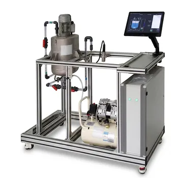
How Does Friction Factor Differ In Laminar Vs Turbulent Flow? Lab Experiment Guide

The friction factor’s dependency reveals the hidden physics of flow. On a fluid mechanics training unit, the friction factor (f) behaves fundamentally differently in laminar and turbulent regimes because of how the flow interacts with the pipe wall. In laminar flow, (f) is a pure function of the Reynolds number (Re), given exactly by (f = 64/\text{Re}), and pipe roughness has absolutely no influence. In turbulent flow, the friction factor becomes a complex function of both Re and the pipe’s relative roughness (\epsilon/D), and surface imperfections suddenly dominate the resistance to flow.

The laminar regime hides pipe roughness behind a thick sublayer, making friction predictable from Re alone. The turbulent regime strips that layer away, forcing the friction factor to depend on both flow momentum and wall texture—a contrast every pilot‑plant experiment must demonstrate.

The Physical Foundation: Why Flow Regime Dictates Friction Factor Behavior

The Laminar Regime: A World of Smooth, Ordered Motion

In laminar flow, fluid moves in organized, parallel layers with very little cross‑mixing.

The laminar boundary layer is thick enough to submerge even the microscopic peaks on a commercial pipe wall. The main flow never “feels” the roughness; the wall appears hydraulically smooth.

This gives rise to the clean analytical result (f = 64/\text{Re}), derived directly from the Hagen–Poiseuille equation. On a training unit, when you measure pressure drop at low flow rates, every data point will land directly on that theoretical line.

The Turbulent Regime: Chaos Exposes the Pipe’s True Face

As the Reynolds number climbs, the laminar sublayer thins dramatically.

Eventually the sublayer becomes thinner than the height of the wall’s micro‑protrusions. Those irregularities now protrude into the chaotic core flow, creating form drag that adds to the viscous friction.

The friction factor here can no longer be expressed by a simple formula. It becomes a function of both Reynolds number and relative roughness ((\epsilon/D)). In practice, students use the Moody chart or iterative equations like Colebrook to see that, at very high Re, (f) flattens and depends almost entirely on the pipe’s roughness.

Experimental Validation on a Training Unit

From Pressure Drop to Friction Factor

A typical experiment measures the head loss ((h_f)) across a straight test section with a known diameter and length.

Using the Darcy–Weisbach equation, (h_f = f \frac{L}{D} \frac{V^2}{2g}), you calculate the experimental friction factor. Simultaneously, you determine Re from the volumetric flow rate.

Plotting (f) versus Re on a log–log scale immediately reveals the two regimes. Laminar points collapse onto the 64/Re line, while turbulent points trace a curve whose position depends on the pipe’s relative roughness.

Visualizing the Transition

The transitional zone (roughly Re 2000‑4000) is a chaotic window where the friction factor can spike unpredictably.

In this region, the flow swings between laminar and turbulent patches, making pressure‑drop measurements highly scattered. Demonstration of this erratic behavior teaches students why industrial piping systems are deliberately designed to stay well away from the critical Reynolds number.

Understanding the Trade‑offs

Limitations of Theoretical Correlations

The laminar relation (f = 64/\text{Re}) is exact only for fully developed, steady, isothermal flow in long, straight pipes. In the short runs and measurement zones of a lab unit, entrance effects can cause deviations.

Turbulent correlations like Colebrook are implicit and require iterative solutions. Experimental scatter, driven by pressure‑sensor resolution and minor air pockets, often masks the fine differences between theoretical curves at moderate roughness.

Pitfalls in Experimental Setup

Flow development length is a critical, often overlooked requirement. Without sufficient straight pipe upstream (typically 30‑50 diameters for turbulent flow, or (0.06,\text{Re},D) for laminar), the velocity profile is not fully established, and measured friction factors will be inaccurate.

At low laminar flow rates, differential‑pressure transmitters or manometers may operate near their resolution limit. Even small vibrations or trapped bubbles in the impulse lines can produce misleading values, so careful set‑up and de‑aeration are essential.

Making the Right Choice for Your Experiment

Your approach to a friction‑factor lab should directly follow your teaching goal.

If your primary focus is demonstrating fundamental principles: Operate clearly in the laminar range (Re < 2000) to confirm the simple (64/\text{Re}) line, then push into the fully rough turbulent zone (high Re) to isolate roughness effects.
If your primary focus is characterizing a specific pipe: Collect data across a wide Re range, use iterative solvers to fit the Colebrook equation, and back‑out the pipe’s equivalent sand‑grain roughness. Compare this value to standard tables as a measure of wall condition.
If your primary focus is illustrating design implications: Force students to calculate required pump head using both laminar and turbulent assumptions for the same flow rate. The often enormous difference immediately conveys why misidentifying the flow regime can lead to undersized pumps or excessive energy costs.

Mastering this experimental dichotomy turns a simple friction factor measurement into a durable, intuitive grasp of how flow state governs hydraulic design.

Summary Table:

Parameter	Laminar Flow Regime	Turbulent Flow Regime
Flow Characteristics	Organized, parallel layers	Chaotic, cross-mixing
Friction Factor ($f$)	$f = 64/\text{Re}$	Function of $\text{Re}$ and $\epsilon/D$
Key Influencing Factors	Reynolds number (Re) only	Re and Relative Roughness ($\epsilon/D$)
Wall Roughness Effect	Negligible (submerged by sublayer)	Significant (exposed by thin sublayer)
Experimental Plot	Collapses onto $64/\text{Re}$ line	Follows Moody chart curves

Bring Fluid Mechanics Theory to Life in Your Lab

Looking to equip your students or researchers with high-accuracy experimental tools? LABPARK provides premium Educational and Vocational Unit Operations Pilot Plants in chemical engineering, bioprocess & biotech, and environmental & water treatment.

Our advanced training units help universities, research institutes, and enterprises bridge the gap between fluid mechanics theory and practical industrial application.

Contact LABPARK today to discover the ideal pilot plant solutions for your laboratory and academic programs!