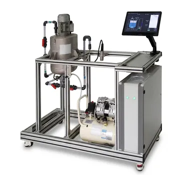
How To Demonstrate Rapid Vs Slow Valve Closure? Clear Water Hammer Transient Experiments For Engineering Labs.

The behavioral transition from rapid to slow valve closure is experimentally demonstrated by systematically varying the closure time of an actuated valve and capturing the pressure signature until the closure duration exceeds the pipe's critical wave-return period. By configuring a fluid mechanics pilot plant with a long straight pipe, a high-speed pressure transducer, and a programmable control valve, educators can directly visualize the moment the pressure wave collapses from a sharp, high-magnitude spike into a series of lower-magnitude oscillations.

The entire demonstration hinges on a single physical constant: the pipe period, defined as the time it takes a sonic wave to travel from the valve to the upstream reservoir and back ($T_r = 2L/c$). If the valve closes faster than this round-trip time, the destructive potential of the water hammer is fully realized. If it closes slower, the returning unloading wave safely "catches" the closure, neutralizing the peak pressure rise.

The Physics Behind the Threshold

Before writing a lab procedure, students must first calculate the theoretical boundary that governs the experiment. This turns a qualitative observation of pressure spikes into a quantitative prediction.

Defining the Pipe Period ($2L/c$)

The critical time threshold is not an arbitrary valve setting—it is a physical property of the test rig. It depends solely on the pipe length ($L$) and the acoustic wave speed ($c$) of the fluid. For water in a rigid steel pipe, $c$ is approximately 1,000–1,400 m/s. A 50-meter pipe therefore has a pipe period of roughly $100/1,200 \approx 0.083$ seconds (83 milliseconds).

The Governing Principle: Wave Interference

The catastrophic pressure rise results from the stagnation of fluid momentum. When a valve shuts, the upstream fluid compresses against it, generating a high-pressure wave traveling upstream. Rapid closure traps this energy. Slow closure allows the negative reflection (the unloading wave) from the upstream reservoir to return to the valve while it is still partially open, cancelling the buildup through destructive interference.

Instrumenting the Demonstration

Standard flow loops are incapable of showing this phenomenon due to sensor lag. A successful demonstration relies on high-speed data acquisition and precision actuation.

Essential Sensor Hardware

To capture a transient event lasting less than a tenth of a second, the system must utilize piezoresistive or piezoelectric pressure transducers mounted flush with the pipe wall immediately upstream of the closure valve. Standard industrial transmitters with 100-millisecond response times will completely miss the rapid-closure spike.

High-Speed Data Acquisition Systems

The acquisition hardware is equally critical. A sampling rate of at least 1,000 Hz (1 kHz) is required to reconstruct the sharp "water hammer" waveform accurately. Slower logging will alias the signal, making a catastrophic rapid-closure event look falsely identical to a harmless slow oscillation.

Visualizing the Two Waveform Regimes

The core learning outcome is the visual distinction on the oscilloscope or software dashboard. When plotted, the pressure profiles reveal the stark difference in system stress.

The Rapid Closure Profile ($t_{close} < 2L/c$)

When the valve closure time is set shorter than the pipe period, the pressure trace shows a near-instantaneous vertical spike. The maximum theoretical pressure rise ($p' = \rho c V$) is fully achieved, as the fluid velocity drops from the initial steady-state value ($V$) to zero without the relief valve having time to intervene. The waveform often resembles a square wave or a water-hammer "staircase" pattern due to repeated wave cycling.

The Slow Closure Profile ($t_{close} > 2L/c$)

By incrementally increasing the valve stroking time via the actuator control software, the sharp spike begins to truncate. Once the closure time safely exceeds $2L/c$, the peak pressure rise is drastically reduced. The pressure climbs gradually, plateaus at a much lower value, and settles without the violent resonant banging characteristic of rapid closure.

Designing the Experimental Procedure

Students should not simply press a button; they must predict the failure point. The experiment should be framed as a validation of the Joukowsky equation ($p' = \rho c V$) and wave theory.

Step 1: Establish the Steady-State Baseline

Run the pump at a constant speed to achieve a steady flow velocity ($V$). Record the static pressure to establish the datum line. The transient pressure rise will be measured as the deviation above this operating pressure.

Step 2: Perform the "Step-Change" Closure Sequence

Program the control valve to close in decreasing increments, starting from a very safe slow closure (e.g., 1 second) and moving toward speeds faster than the calculated $2L/c$ boundary. This sweep must start slow to avoid damaging the system on the first run with an unexpected rapid spike.

Step 3: Overlay and Interpret the Curves

The most powerful pedagogical moment is the superposition plot. Overlaying the pressure traces for $t_{close} = 500 ms$, $100 ms$, $84 ms$ (the threshold), and $40 ms$ shows a family of curves where the peak amplitude becomes asymptotic to the theoretical maximum as the valve speed crosses the threshold.

Understanding the Trade-offs

Demonstrating the violent nature of rapid closure in a classroom setting carries inherent practical risks that must be balanced against educational value.

Managing Acoustic Noise and Vibration

True rapid closure in a rigid pipe often produces a loud, gunshot-like bang. This can be alarming or even physically damaging to the test rig. To mitigate this without destroying the physics, you can introduce a small air chamber or deliberately use a slightly flexible hose section to dampen the highest frequencies while still preserving the clear visual distinction on the pressure trace.

The Pressure Rise vs. Flow Rate Paradox

For the rapid-closure pressure spike ($\rho c V$) to be visually dramatic, the initial flow velocity ($V$) must be high. However, high velocity induces high friction loss, which distorts the ideal square-wave profile. A trade-off exists: use a pipe material with low acoustic wave speed ($c$), which simultaneously increases the pipe period ($2L/c$) and makes the threshold slower and easier to capture, while keeping flow velocity modest to avoid steady-state noise.

Making the Right Choice for Your Lab Setup

The decision on how to demonstrate this depends entirely on your available hardware and safety constraints.

If your primary focus is precise theoretical validation: Use a rigid stainless steel pipe, a high-speed servo-driven ball valve with positional feedback, and an acquisition rate above 10 kHz. Prioritize wave reflection clarity over safety.
If your primary focus is operator safety and basic visualization: Select a shorter, slightly flexible pipe and a pneumatic actuator. Accept some wave attenuation in exchange for a quieter demonstration that still clearly shows the amplitude reduction at the $2L/c$ threshold.
If your primary focus is destructive testing awareness: Configure the system to intentionally trap the transient by performing rapid closure first. Show the danger, then immediately run the slow closure scenario to show how a simple operational adjustment removes the destructive load.

By forcing the valve closure time to cross the calculated $2L/c$ boundary and capturing the resulting pulse truncation, you convert an abstract mathematical threshold into an unforgettable physical lesson on system dynamics.

Summary Table:

Parameter	Rapid Closure ($t_{close} < 2L/c$)	Slow Closure ($t_{close} > 2L/c$)
Pressure Profile	Near-instantaneous vertical spike (square/staircase wave)	Gradual climb, lower plateau, smooth settling
Wave Interference	Energy trapped; no unloading wave relief	Unloading wave cancels buildup (destructive interference)
Max Pressure Rise	$p' = \rho c V$ (Theoretical maximum reached)	Drastically reduced; peak pressure truncated
System Impact	High vibration, loud banging, potential damage	Safe, quiet, minimal system stress

Enhance Your Engineering Curriculum with LABPARK

Bring fluid mechanics and complex transient physics to life in your lab. LABPARK provides state-of-the-art Educational and Vocational Unit Operations Pilot Plants in chemical engineering, bioprocess & biotech, and environmental & water treatment tailored for universities, research institutes, and enterprises.

Our custom-built pilot plants are equipped with high-speed data acquisition and precision instrumentation, enabling students and researchers to safely analyze fluid behavior, water hammer dynamics, and control system responses.

Ready to upgrade your laboratory capabilities? Contact LABPARK today to discuss your custom pilot plant configuration!