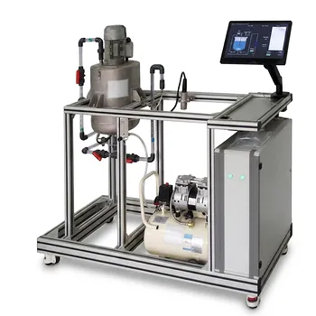
How Do Rtd Measurements Differ In Homogeneous Vs. Heterogeneous Reactors? Key Unit Ops Insights

While a homogeneous reactor’s RTD is essentially indifferent to the tracer you choose, a heterogeneous reactor’s RTD is a fingerprint of that specific tracer’s chemical and physical interactions with the catalyst or phase boundaries. In teaching-unit operations equipment, this means the same physical reactor can yield completely different residence-time distributions depending on whether you inject a dye, a non-adsorbing gas, or an isotopically labeled reactant – and interpreting those differences is the entire point of the experiment.

The central insight for educational RTD work is this: In homogeneous systems (CSTRs, tubular reactors in turbulent flow), the RTD is a pure fluid-dynamic signature that is virtually identical for all chemical species, making simple tracers perfectly acceptable. In heterogeneous systems (packed-bed catalytic reactors, gas-liquid columns), the RTD becomes a species-specific convolution of flow, surface interaction, and mass transfer – so naïve tracer choice can give you a dangerously misleading picture of true reactant behavior.

Why the Reactor Configuration Dictates the Meaning of an RTD Curve

The Homogeneous Case: A Clean Fluid-Dynamic Fingerprint

In a homogeneous liquid or gas-phase reactor operating under turbulent conditions, all molecular species are swept along by the same macroscopic flow patterns.

There is no phase boundary to selectively slow down one molecule versus another.

As a result, the residence-time distribution you measure with a conductivity probe and a salt tracer, for instance, is functionally identical to the RTD the actual reactants would experience. This is why CSTR and tubular reactor pilot plants are forgiving – the tracer’s identity does not matter. You can use any inert substance that is easy to detect, and the resulting f(t) or F(θ) curve directly represents the degree of backmixing, bypassing, or dead zones in the vessel.

Students learn core mixing concepts – like the coefficient of variation narrowing from 1 to 1/√n as identical CSTRs are placed in series – using data that directly reflects physical reality. Standard RTD theory, which assumes homogeneity, applies with minimal error, so the educational transition from a single tank to ten stirred tanks in series smoothly demonstrates the approach to plug-flow behavior.

The Heterogeneous Case: When the Tracer Becomes a Reactant Surrogate

A packed-bed catalytic converter or a gas-liquid absorption column fundamentally changes the game. Here, reactants, intermediates, and products each have unique affinity for the solid catalyst surface or the second phase.

An inert tracer gas, such as helium, might zip through the packed bed, bypassing pores entirely and indicating only the interstitial velocity distribution.

A strongly adsorbing reactant, however, will spend significant time inside catalyst pores – a delay completely invisible to the helium. That extra “chemical residence time” is the reactor’s true performance driver, and its RTD will look dramatically different, often exhibiting a long tail or a shifted mean residence time.

This is not a defect; it is a feature. The difference between a non-adsorbing tracer’s RTD and an isotopically marked reactant’s RTD allows students to deconvolute flow maldistribution from true kinetic hold-up. The tracer’s response becomes a probe of adsorption, desorption, and pore diffusion, not just mixing. The key lesson: in heterogeneous educational equipment, no single RTD tells the whole story.

The Critical Role of Tracer Selection

Your experimental objective dictates the tracer. If you want to diagnose if a packed bed has poor flow distribution causing hot spots or bypassing, you deliberately choose a non-adsorbing, non-condensing tracer. This clean fluid-dynamic baseline isolates the physical flow.

If you need to understand the true conversion dynamics and predict the yield of a specific reaction, you must use an isotope-marked reactant or a tracer that mimics that reactant’s surface interactions. Anything less, and your measured RTD might be off by orders of magnitude in terms of mean contact time.

This duality is the core educational takeaway: the instrument gives you a number, but the physical meaning of that number is entirely determined by whether your system respects the homogeneous assumption or actively violates it.

How RTD Metrics Manifest Differently in Each Configuration

Visualizing the Difference Through Cumulative and Density Functions

Plotting the dimensionless cumulative distribution F(θ) and the density function f(θ) makes the distinction concrete.

In a homogeneous tubular reactor, the f(θ) curve for any species is essentially identical. Any broadening relative to a perfect PFR spike reflects axial dispersion caused by turbulence and velocity gradients – a purely physical spreading that affects all molecules equally.

In a heterogeneous packed bed, superimpose the f(θ) curves for an inert tracer and a reactive species. The inert tracer’s curve may be relatively narrow, while the reactive species’ curve exhibits a pronounced tail and a mean shifted to longer dimensionless time. That lag is not due to poor fluid mixing; it is the residence time inside the stationary phase, a phenomenon completely absent in the homogeneous case.

Variance as a Diagnostic Tool with a Caveat

The RTD variance is a single-number metric that students use to quantify dispersion. A variance near zero suggests plug flow; a high variance suggests backmixing or channeling.

In homogeneous systems, this mapping holds neatly. In heterogeneous systems, however, a high variance can have two completely different origins: genuine fluid-dynamic channeling or slow intraparticle diffusion. A large variance measured with an inert tracer likely indicates a packing problem. The same large variance measured with a reactant-mimicking tracer might indicate the catalyst’s pore structure is performing exactly as designed, providing ample surface area for reaction. Students must learn to cross-reference the tracer identity with the variance value rather than taking it at face value.

Understanding the Trade-offs and Common Pitfalls

The Homogeneous Assumption Trap

The biggest risk in an educational lab is that students will apply the simple, elegant RTD theory learned in a homogeneous CSTR or PFR module directly to a heterogeneous pilot plant without adjusting their mental model.

Standard RTD textbook relationships are rigorously derived for single-phase, non-interacting flow. When you bring those formulas to a catalytic reactor, the derived parameters (like the dispersion number or tanks-in-series equivalent) no longer represent pure mixing – they conflate fluid dynamics with mass-transfer resistances. Recognizing this boundary is precisely why pilot-scale heterogeneous experiments exist.

The Tracer Is the Lens, Not the Object of Study

A related pitfall is fixating on the tracer’s behavior as if it were the truth about the reactant. If a student uses a non-adsorbing tracer in a strongly adsorbing system and concludes the reactor has “too little hold-up,” they are seeing a true statement about the tracer, not about the reactant.

The defense against this error is to run comparative RTD experiments: one with an inert tracer, one with a slightly adsorbing or isotopically labeled species. The gap between the two curves is the practical measure of adsorption capacity and mass-transfer limitation – the real data you need for reactor design and scale-up.

How to Apply This to Your Teaching Unit or Pilot Plant

After understanding these fundamental differences, align your experimental protocol with your learning objective. Tailor your approach as follows:

If your primary focus is teaching ideal reactor behavior and the fundamentals of non-ideal mixing: Use a homogeneous CSTR or tubular reactor pilot plant with a simple, reliable tracer. The tracer’s identity is irrelevant, and the clean data will showcase the transition from backmixed to plug flow.
If your primary focus is diagnosing catalyst bed maldistribution or packing quality: Select a non-adsorbing tracer that has zero affinity for the solid phase. The RTD will isolate physical flow faults such as channeling or dead zones without being clouded by surface chemistry.
If your primary focus is studying actual reaction dynamics, conversion prediction, or scale-up feasibility: Use an isotope-marked reactant or chemically analogous tracer. Accept that the resulting RTD represents a combined flow-and-kinetic signature, and compare it against a non-adsorbing baseline to extract the contributions of adsorption and pore diffusion.
If your primary focus is analyzing multiphase holdup and mass transfer: Inject different tracers tailored to each phase and observe their distinct RTDs. The differences in mean residence time and tail shape directly quantify phase interchange and transport resistances.

Ultimately, the RTD experiment in educational unit operations equipment stops being about simply “finding the mixing pattern” and becomes a lesson in model awareness: the physical chemistry of your tracer always defines what you are actually measuring, and in heterogeneous configurations that choice is everything.

Summary Table:

Feature	Homogeneous Configuration	Heterogeneous Configuration
Primary Driver	Pure fluid dynamics (mixing, bypassing)	Flow, surface adsorption, & mass transfer
Tracer Selection	Indifferent (any inert tracer works)	Highly dependent (adsorbing vs. non-adsorbing)
Variance Meaning	Indicates physical dispersion/channeling	Conflates physical mixing with pore diffusion
Educational Focus	Teaching ideal reactor mixing concepts	Diagnosing mass-transfer limits & kinetics

Upgrade Your Chemical Engineering Lab with LABPARK

To effectively teach complex reactor dynamics like RTD, students need reliable, high-quality hardware. LABPARK designs and supplies premium Educational and Vocational Unit Operations Pilot Plants in chemical engineering, bioprocess & biotech, and environmental & water treatment.

We help universities, research institutes, and enterprises bridge the gap between theory and practical application with robust, industry-grade systems.

Contact LABPARK today to explore our pilot plant configurations and request a quote!