How Can Bench-Scale Filtration Studies Using The Vmax Model Be Integrated Into Bioprocess Lab Courses?

The fastest way to demystify industrial filter sizing is to have students run a 40 cm² test and then calculate the area needed for a 2,000-liter bioreactor. By conducting a constant‑pressure flow‑decay study with a bench‑scale capsule filter, plotting the reciprocal relationship ( t/V ) versus time, and extracting the maximum filterable volume per unit area (( V_{max} )), students can directly apply a proven scaling equation to compute the minimum required filtration area for any target batch. This hands‑on module transforms an abstract engineering concept into a concrete, teachable design workflow.

The core takeaway: A ( V_{max} )-based lab class bridges the gap between textbook filtration theory and real bioprocess design. Students learn to collect flow‑decay data, perform a linear regression for ( V_{max} ), and then use the scaling equation ( A_{min} = V_B \left( \frac{1}{V_{max}} + \frac{1}{J_i t_B} \right) ) to size a production filter—complete with a 50% safety margin. The exercise builds critical thinking about capacity limits, flux constraints, and the non‑linear nature of scale‑up.

The Pedagogical Gap That a Filtration Lab Fills

Traditional bioprocess courses excel at teaching theoretical flux models, yet students often struggle to translate those models into a filter area number that a bioreactor actually demands. A bench‑scale ( V_{max} ) experiment closes that gap by making the entire scale‑up calculation a tangible, data‑driven exercise.

Moving from Theory to Predictive Design

Textbook equations describe flux decline due to pore plugging or cake formation, but they rarely give a direct path to sizing. The ( V_{max} ) model does exactly that: it captures the fouling behavior of a specific feed‑filter pair in a single, experimentally accessible parameter.

By generating their own ( V_{max} ) value, students see that filter sizing is not guesswork. It is a reproducible measurement followed by a clear algebraic step—exactly the mindset they need for process development.

Building an Intuition for Filtration Capacity

When students record how the flow rate decays over an hour and then see that data collapse into a single ( V_{max} ) number, they internalize what “maximum filterable volume” means. They learn that a filter has a finite throughput capacity, not just a nominal pore size, and that this capacity depends on both the membrane and the feed stream.

This physical intuition is difficult to convey through lectures alone. The act of watching flow dwindle and then quantifying its limit cements the concept permanently.

Designing the Experiment: From Hardware to Data Collection

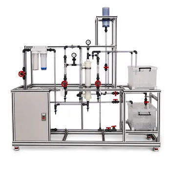
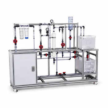
The lab setup is deliberately simple, so that the intellectual content—data interpretation and scale‑up—remains the focus. A small capsule filter, a pressurized feed vessel, and a balance are all that is required.

A Minimalist Yet Realistic Setup

A 40 cm² capsule filter (commonly a 0.2 µm sterilizing‑grade membrane) is connected to a pressurized feed reservoir. The feed can be a model protein solution, a yeast suspension, or clarified cell culture fluid—any liquid that causes a measurable flow decline within a typical lab period.

Constant pressure is maintained throughout the run (e.g., 1.0 bar), and the cumulative filtrate mass is recorded at regular intervals. Converting mass to volume gives the raw data for analysis.

Capturing the Right Data Points

The initial flux falls quickly, so early readings must be frequent—every 10–15 seconds during the first few minutes. As the flow plateaus, the interval can be extended to one minute or more.

The experiment runs until the flux becomes very low or until a total filtrate volume is reached that clearly defines the slope in the ( t/V )-vs‑time plot. This typically requires 30–60 minutes, easily fitting into a standard laboratory session.

Extracting Vmax: The Power of the t/V Plot

The breakthrough moment for students comes when they realize that a simple linear plot reveals the ultimate filtration capacity of the system. The analysis method is robust and requires only elementary spreadsheet skills.

Performing the Linear Regression

Students compute the ratio ( t/V ) for each time point and plot it on the y‑axis against ( t ) on the x‑axis. For many constant‑pressure dead‑end filtrations, this plot yields a straight line after an initial transient.

The slope of that line is ( 1/V_{max} ), and the intercept is ( 1/(J_i A) ). A basic linear regression in Excel or any plotting software instantly delivers the two most important design parameters from a single graph.

What Vmax Truly Represents

( V_{max} ) is the maximum filterable volume per unit membrane area—the theoretical volume that the filter would process if it could run to complete plugging. It is not a direct measure of flux, but of throughput capacity.

A high ( V_{max} ) means the feed is well‑suited to the membrane and the filter will process a large volume before fouling. A low ( V_{max} ) indicates rapid plugging, signaling that a different membrane or a multistage filtration scheme may be needed. This single number thus becomes a powerful comparative tool.

Scaling Up: From Vmax to Minimum Area

With ( V_{max} ) in hand, the lab module pivots to its most career‑relevant question: “Given this feed, how big a filter does our 500‑liter batch need?” The answer comes from a straightforward scaling equation.

The Design Equation in Practice

The minimum required filtration area, ( A_{min} ), is calculated as:

[ A_{min} = V_B \left( \frac{1}{V_{max}} + \frac{1}{J_i , t_B} \right) ]

Here ( V_B ) is the target batch volume, ( t_B ) is the allowable processing time (often a few hours), and ( J_i ) is the initial flux measured during the bench‑scale test. Students plug in their experimental values and immediately see a real‑world area estimate—transforming their lab data into a process engineering decision.

Embedding a Safety Margin for Realism

To prepare students for industrial practice, the final calculated area is multiplied by a 1.5× safety factor. This margin accounts for feed‑property variability, scale‑up inaccuracies, and the practical reality that operators never run a filter at its absolute capacity limit.

Students then compare this safety‑adjusted area to commercially available filter capsule sizes, learning how to navigate product catalogs and select the next standard size up. This step turns a theoretical calculation into a manufacturable choice.

Understanding the Trade-offs and Limitations of the Vmax Model

A trustworthy educational experience acknowledges that no model is perfect. Discussing the model’s boundaries teaches students healthy skepticism and prevents blind reliance on any single measurement.

Assumptions That Can Break Down

The ( V_{max} ) model assumes a constant‑pressure operation and a stable fouling mechanism throughout the run. If the feed contains components that form a compressible cake or that change their fouling behavior with time, the ( t/V ) plot may deviate from linearity, and the extracted ( V_{max} ) loses predictive accuracy.

Similarly, the model treats the entire filter as a single lumped system, ignoring local variations or non‑uniform flow. In large production filters, flow distribution can become uneven, making the simple area linearity less reliable.

Why One Test is Not Enough

A single bench‑scale run gives a point estimate of ( V_{max} ) for one set of conditions. Real feeds change from batch to batch, and even minor shifts in pH or temperature can alter fouling rates. Students should therefore repeat the experiment with altered process parameters or mock feed variability to appreciate the range of possible outcomes.

The arbitrary 50% safety factor, while pragmatic, is a rule of thumb. Industries often refine this margin based on statistical analyses of many historical runs, a nuance that an advanced lab can explore.

Scale‑Up as a Learning Opportunity, Not a Guarantee

The bench‑to‑production translation should be framed not as an exact prediction, but as a rapid exercise in order‑of‑magnitude sizing and risk identification. A calculated 1.2 m² minimum area with a 1.8 m² safety factor tells an engineer, “A 2.5 m² capsule is likely sufficient, but a 3.2 m² option gives headroom if the feed turns problematic.”

This mindset prepares students for the iterative, at‑times uncertain reality of bioprocess development.

Making the Lab Module a Success: Actionable Recommendations

Every educational setting has different priorities. Align the experiment’s complexity and discussion points with your primary learning outcome to maximize impact.

If your primary focus is reinforcing mass‑transfer and fouling principles: Emphasize the theory behind the ( t/V ) linearization and have students derive the slope‑( V_{max} ) relationship. Discuss why the model fits constant‑pressure dead‑end filtration and where it diverges from cake‑filtration models.
If your primary focus is hands‑on experimental and data‑analysis skills: Prioritize meticulous data collection, error analysis in the linear regression, and spreadsheet proficiency. Require students to quantify the uncertainty in ( V_{max} ) and its effect on calculated area.
If your primary focus is preparing students for industrial process design: Add a “select‑the‑capsule” step using real vendor catalog data. Have students justify their safety margin choice and present a filtration‑cost estimate for the scaled‑up batch, tying the experiment directly to operational expenditure.

Transforming a 40 cm² flow‑decay test into a full‑scale filter sizing exercise gives students a compact, repeatable, and deeply instructive window into bioprocess design. With a single lab session, they move from measuring volumes to making process decisions—a leap that stays with them long after the glassware is put away.

Summary Table:

Parameter	Symbol	Definition & Scale-up Role
Max Filterable Volume	$V_{max}$	Theoretical throughput limit per unit area before fouling
Initial Flux	$J_i$	Starting flow rate per unit area of the filter
Target Batch Volume	$V_B$	Total volume requiring filtration in production
Allowable Time	$t_B$	Target processing time for the full batch
Minimum Area	$A_{min}$	Calculated base filtration area: $V_B(1/V_{max} + 1/(J_i t_B))$

Bring Industrial Scale-Up into Your Laboratory

Equip your students with the practical skills needed for modern bioprocess development. LABPARK provides premium Educational and Vocational Unit Operations Pilot Plants in chemical engineering, bioprocess & biotech, and environmental & water treatment for universities, research institutes, and enterprises.

Ready to upgrade your lab curriculum with hands-on scale-up equipment? Contact LABPARK today to request a quote or custom consultation!