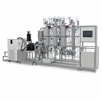
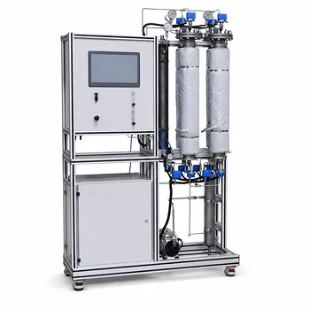
The dynamic time constant and static gain of a gas-pressure control pilot plant are determined primarily by vessel storage capacity, gas properties, and the linearized flow resistance of the valves. For an ideal gas, storage capacity increases with vessel volume and decreases with absolute temperature, while the valve resistance depends on how strongly inlet or outlet flow responds to pressure drop. The static gain additionally depends on the selected input, such as valve opening or supply pressure, and on the steady-state operating point.

Vessel volume and gas compressibility determine how much gas must accumulate to change pressure; valve flow characteristics determine how quickly that pressure changes. The time constant describes response speed, while the static gain describes the magnitude of the final pressure change for a given input change.

How Gas Storage Determines the Dynamic Response

Vessel Volume and Gas Compressibility

For a rigid vessel containing an ideal gas, the pressure-storage relationship follows from:

[ PV = nRT ]

At approximately constant temperature, a change in the number of moles produces a pressure change according to:

[ \Delta P = \frac{RT}{V}\Delta n ]

Thus, a larger vessel requires more gas accumulation or removal to produce the same pressure change. It therefore has greater storage capacity and generally responds more slowly.

Process Temperature

Temperature affects the pressure response through the gas constant relationship. At a fixed vessel volume and molar change, higher absolute temperature produces a larger pressure change.

For dynamic analysis, temperature must be treated consistently. If gas temperature changes significantly during filling, venting, or compression, the pressure response may no longer be represented accurately by a constant-temperature model.

Gas Composition and Compressibility

For gases that depart from ideal behavior, the pressure-storage relationship also depends on gas composition and the compressibility factor (Z):

[ PV = ZnRT ]

In that case, the effective storage capacity depends on pressure, temperature, composition, and (Z). Even when the ideal-gas assumption is appropriate, gas composition matters because it can affect density, flow properties, and valve behavior.

How Valve Characteristics Determine the Time Constant

Linearized Valve Resistance

The time constant is governed by the product of storage capacity and flow resistance:

[ \tau_p = C_p R_v ]

For an ideal gas in a rigid, approximately isothermal vessel, the pressure-storage capacity is proportional to:

[ C_p \propto \frac{V}{RT} ]

The valve resistance is obtained by linearizing the flow relation around the operating point. If (F) is the molar or mass flow rate and (\Delta P_v) is the pressure drop across the valve:

[ R_v = \left(\frac{\partial F}{\partial \Delta P_v}\right)^{-1}_{\text{operating point}} ]

Therefore, the time constant depends on:

Vessel volume (V)
Absolute gas temperature (T)
Gas properties and composition
Valve flow coefficient
Valve opening or position
Upstream and downstream pressures
The local slope of the valve flow-pressure characteristic

A valve with a small flow response to pressure-drop changes has high resistance and produces a longer time constant. A valve with a strong flow response has lower resistance and produces a faster pressure response.

Inlet and Outlet Flow Paths

The relevant resistance is not necessarily the resistance of one valve alone. It may include the combined effects of inlet valves, outlet valves, piping, regulators, restrictions, and other flow elements.

For a pressure vessel with both inlet and outlet flows, the effective resistance is determined by how the net flow changes when vessel pressure changes:

[ F_{\text{net}} = F_{\text{in}} - F_{\text{out}} ]

The linearized derivative of this net flow determines the local dynamic resistance seen by the vessel.

Operating-Point Dependence

Gas valves are nonlinear devices. Their flow may depend on pressure ratio, choking conditions, valve position, and the particular valve characteristic.

Consequently, the time constant measured at one pressure and valve opening may not apply at another. A pilot plant is often best represented by a local first-order model whose parameters are identified near the operating condition of interest.

How Static Gain Is Determined

Definition of Static Gain

The static gain is the steady-state change in vessel pressure divided by the change in the selected process input:

[ K_p = \frac{\Delta P_{\text{steady state}}}{\Delta u} ]

where (u) may represent valve opening, controller signal, inlet flow command, or supply pressure.

The gain is therefore not a universal property of the vessel alone. It depends on both the chosen input and the operating point.

Gain for Valve-Opening Changes

For a valve-opening input, the static gain depends on how much the valve changes the steady-state flow balance. In a pressure vessel, the final pressure is reached when inlet and outlet flows are again equal.

A valve with a large change in flow per unit change in opening can produce a larger steady-state pressure change, provided the rest of the system does not offset that change through another flow path.

Gain for Supply-Pressure Changes

If the input is upstream supply pressure, the gain depends on the sensitivity of valve flow to that supply pressure and on the pressure-dependent behavior of the opposing flow path.

The same vessel can therefore have different static gains for a valve-position input and a supply-pressure input.

Relationship to a Step Response

For a first-order approximation:

[ \frac{\Delta P(s)}{\Delta u(s)}

\frac{K_p}{\tau_p s+1} ]

After a step change in input, the pressure approaches its final value according to:

[ \Delta P(t)

K_p\Delta u \left(1-e^{-t/\tau_p}\right) ]

The pressure has reached approximately 63.2% of its final change after one time constant and approximately 98% after four time constants.

The Role of Control-Loop Configuration

Controlled and Manipulated Variables

The calculated parameters depend on what the control system measures and manipulates. Common choices include:

Controlled variable: vessel pressure
Manipulated variable: inlet-valve opening
Disturbance: outlet demand or supply-pressure fluctuation

Changing the manipulated variable changes the process gain. A model identified using inlet-valve position cannot automatically be used unchanged for an outlet-valve position.

Sensor and Actuator Effects

The vessel and valves define the dominant process dynamics, but pressure sensors, signal filtering, actuator delays, and controller output limits can add additional dynamics.

These effects should be separated from the process time constant when possible. Otherwise, the identified (\tau_p) may include measurement or actuator delay rather than representing the gas-storage process alone.

Understanding the Trade-offs

Larger Vessels Improve Damping but Slow Response

A larger vessel provides greater gas storage and can reduce the pressure impact of short disturbances. Its increased storage capacity also produces a longer response time when valve resistance is unchanged.

This creates a practical trade-off between pressure buffering and control speed.

High Valve Resistance Improves Regulation but Increases Lag

Restrictive valves or flow paths reduce the rate at which gas enters or leaves the vessel. This can make the process easier to regulate in some operating ranges, but it also increases the time required for pressure to respond.

Excessive resistance can make the loop sluggish and limit achievable control performance.

Nonlinearity Limits a Single Fixed Model

The ideal first-order model is a local approximation. Valve flow characteristics, pressure ratios, gas temperature, and flow regime can change with operating conditions, causing both (K_p) and (\tau_p) to vary.

Using one parameter pair over a wide operating range can lead to poor PID tuning or inconsistent response.

Thermal Effects Can Distort Pressure Measurements

Filling, venting, throttling, or compression can change gas temperature. Because pressure depends directly on temperature, an observed pressure change may reflect both gas accumulation and thermal effects.

When temperature variations are significant, pressure and temperature should be measured together, and an energy balance may be needed.

Making the Right Choice for Your Goal

Use a step test near the intended operating point: record the input change, steady-state pressure change, and response time, then estimate (K_p) from the final pressure change and (\tau_p) from the 63.2% response point.

If your primary focus is faster pressure response: Reduce effective storage capacity or flow resistance, while checking that the valves and piping can handle the required flow safely.
If your primary focus is pressure buffering: Increase vessel volume or effective gas storage, accepting a longer dynamic time constant.
If your primary focus is PID tuning: Identify (K_p) and (\tau_p) using the same manipulated variable and operating range used by the controller.
If your primary focus is accuracy across changing conditions: Repeat parameter identification at multiple pressures, temperatures, and valve positions or use gain scheduling.
If your primary focus is diagnosing unexpected dynamics: Separate vessel, valve, sensor, actuator, and thermal contributions before changing controller settings.

A reliable pressure-control model comes from treating vessel storage, valve flow sensitivity, and operating conditions as one connected system.

Summary Table:

Parameter	Effect on Dynamic Time Constant	Effect on Static Gain
Vessel volume	Larger volume increases storage and slows pressure response	Influences the pressure change required to reach a new steady state
Gas temperature	Changes pressure-storage behavior; thermal changes can add dynamics	Affects the final pressure response
Gas composition and compressibility	Alters density, flow behavior, and effective storage	Changes flow sensitivity and steady-state response
Valve flow coefficient and opening	Higher resistance generally increases the time constant	Determines how strongly pressure responds to valve-position changes
Inlet and outlet flow paths	Combined net-flow resistance controls response speed	Sets the final pressure balance
Upstream and downstream pressure	Changes valve flow regime and local resistance	Affects sensitivity to supply-pressure changes
Selected process input	Determines which gain is identified	Gain may differ for valve opening, flow command, or supply pressure
Operating point	Causes local values of gain and time constant to vary	Nonlinear valve behavior makes gain operating-point dependent
Sensor, actuator, and thermal effects	Can add delay or apparent process dynamics	May distort the measured steady-state response

Need reliable pressure-control training and pilot-plant data for your next project? Contact LABPARK to discuss Educational and Vocational Unit Operations Pilot Plants for gas-pressure control and related chemical engineering applications. LABPARK helps universities, research institutes, and enterprises evaluate vessel storage, valve characteristics, gas behavior, and operating-point effects through practical, configurable systems. We also provide pilot plants for bioprocess and biotech operations and environmental and water treatment, helping your team improve laboratory teaching, process research, scale-up studies, and industrial training with equipment matched to your technical goals.