How Is The Direction And Driving Force Of Mass Transfer Determined In A Gas Absorption Unit Operations Pilot Plant?

The direction of mass transfer is determined by a single comparison: the actual phase composition versus its equilibrium value.

If the actual gas-phase mole fraction (y) is greater than the equilibrium value (y*), the solute transfers from the gas to the liquid, and absorption occurs. If y is less than y*, the solute transfers from the liquid to the gas, and desorption (or stripping) occurs. The driving force is the magnitude of this deviation from equilibrium, typically quantified as a concentration difference (Δy or Δx) or a partial pressure difference (Δp). A larger deviation creates a more powerful driving force, leading to a faster mass transfer rate.

Determining the direction and driving force in a gas absorption pilot plant is fundamentally an analysis of distance from equilibrium. The system's natural drive is to close the gap between its current state and its equilibrium state. The core practical challenge is not just understanding this principle, but accurately measuring the compositions that define this gap.

The Fundamental Principle: Equilibrium as the Compass

Before any calculation, you must establish the target. The equilibrium relationship for the specific gas-liquid system is the reference point against which all process decisions are made.

Defining the Operational Compass

All mass transfer decisions hinge on a comparison. The system’s natural compass always points toward equilibrium.

Absorption (Gas to Liquid): The system is not at equilibrium and contains more solute in the gas phase than it would at saturation. The natural direction is to push solute into the liquid. This corresponds to y > y* (or x < x*).
Desorption/Stripping (Liquid to Gas): The system contains more solute in the liquid phase than equilibrium allows. The natural direction is to expel solute into the gas phase. This corresponds to y < y* (or x > x*).

Quantifying the Gap: Forms of the Driving Force

The driving force is the numerical expression of the system’s eagerness to move toward equilibrium. Its magnitude directly controls the transfer rate.

You express this force in terms of the phase where the dominant resistance lies. Three common forms are:

Gas-Phase Concentration Difference: Δy = y - y*
Liquid-Phase Concentration Difference: Δx = x* - x
Partial Pressure Difference: Δp = p - p*

A small deviation means the system is near equilibrium and transfer will be slow. A large deviation means the system is far from equilibrium and transfer will be rapid.

The Critical Role of Solubility in Shaping the Driving Force

Not all systems are alike. The solute's solubility dictates where the key resistance—and thus the most significant portion of the overall driving force—resides.

Gas-Film Controlled Systems

Some gases are highly soluble. In these cases, the liquid absorbs the solute with ease, and the bottleneck is on the gas side.

For a system with a high solubility gas (e.g., ammonia in water), the mass transfer resistance is almost entirely in the gas film. The overall mass transfer coefficient approximates the gas-film coefficient (K_G ≈ k_g). To maximize the driving force and the rate of absorption, you must focus on overcoming the gas-side resistance by increasing gas-phase turbulence or velocity.

Liquid-Film Controlled Systems

Other gases are sparingly soluble. The gas may be willing to dissolve, but the liquid struggles to accept it, creating a bottleneck on the liquid side.

For a system with a low solubility gas (e.g., carbon dioxide in water), the resistance is concentrated in the liquid film (K_L ≈ k_l). Here, no amount of gas-phase agitation will dramatically improve the rate. The driving force must be applied by optimizing liquid flow rate, improving liquid distribution, or enhancing packing wettability to overcome the liquid-side resistance.

Practical Measurement in a Pilot Plant

Determining the driving force is not a purely theoretical exercise; it requires connecting the abstract principle to the physical plant's data.

From Measurement to Meaning

A pilot plant’s primary function is to make the invisible visible. Key performance indicators are derived from direct measurements.

By measuring the solute concentration at different heights along an absorption column, you map a concentration profile. These datapoints, combined with mass balance equations, allow you to calculate the overall mass transfer coefficient. Parameters like the volumetric mass transfer coefficient (kLa) are not directly measured but calculated. You can determine kLa by, for instance, measuring dissolved oxygen profiles over time, linking the measured change in concentration back to the driving force that caused it.

Verifying with Operating and Equilibrium Curves

One of the most powerful educational uses of a pilot plant is visualizing this concept. By measuring inlet and outlet solute concentrations under different liquid-to-gas ratios (L_m/G_m), you construct an operating line on a graph against the equilibrium curve.

The distance between the operating line and the equilibrium curve is a direct graphical representation of the driving force. A steep operating line far from the curve indicates a large driving force and allows you to verify design calculations like the Number of Transfer Units (NTU) and Height of a Transfer Unit (HTU), validating methods like the Cornell or Onda correlations under real-world conditions.

Understanding the Trade-offs

A singular focus on maximizing the driving force can lead to poor overall design. The process must be viewed holistically.

The Energy-Purity Trade-off

A very large driving force is achieved by using an excessive amount of pure solvent or a very high gas flow rate. While this accelerates mass transfer, it is often inefficient. You must balance the capital cost reduction (from a smaller column due to faster transfer) against the increased operating costs (from pumping more liquid, larger regeneration units, or higher pressure drops). The optimal point is rarely the one with the maximum possible driving force.

The Danger of Flooding

When you increase gas or liquid velocities to enhance turbulence and the driving force, you approach the column's hydrodynamic limits. Pushing a column beyond its flooding point drastically increases pressure drop, creates unstable operation, and causes a sharp drop in mass transfer efficiency as liquid is held up and entrained. The pursuit of a higher driving force must always respect the column’s hydraulic capacity.

Making the Right Practical Choice for Your Experiment

Your focus depends entirely on the phase system you’ve chosen and the resistance you need to overcome.

If your primary focus is a highly soluble gas like ammonia: Your main lever for influencing the driving force is on the gas side. Increase gas velocity and turbulence to reduce the gas-film resistance.
If your primary focus is a sparingly soluble gas like carbon dioxide: Your energy must be directed toward the liquid phase. Optimize liquid flow rates, ensure perfect liquid distribution, and select packing with high wettability to shrink the liquid-film resistance.
If your primary focus is validating column design: Methodically vary the liquid-to-gas ratio and plot the operating line against the equilibrium curve. The graphical gap between them is your driving force, and its profile allows you to calculate and verify critical design parameters like NTU and HTU.
If your primary focus is simply teaching the principle of mass transfer: Run an experiment to the point of equilibrium. Showing students that the measured concentration difference drops to zero is the most powerful demonstration that equilibrium is the sole determinant of both direction and driving force.

Mastering the operation of a gas absorption pilot plant comes down to seeing beyond the pumps and packing—it’s about learning to visualize and manipulate the invisible thermodynamic gap that governs the process.

Summary Table:

Process Type	Mass Transfer Direction	Driving Force Equation	Controlling Resistance
Absorption	Gas to Liquid (y > y*)	Δy = y - y*	Gas-film (High solubility, e.g., NH3)
Desorption / Stripping	Liquid to Gas (y < y*)	Δx = x* - x	Liquid-film (Low solubility, e.g., CO2)

Bring Chemical Engineering Principles to Life with LABPARK

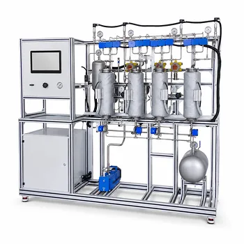
Are you looking to enhance hands-on learning and research in mass transfer? LABPARK provides premium Educational and Vocational Unit Operations Pilot Plants in chemical engineering, bioprocess & biotech, and environmental & water treatment.

Tailored for universities, research institutes, and enterprises, our advanced pilot plants help students and researchers visualize thermodynamic gaps, calculate critical HTU/NTU design parameters, and master gas absorption operations.

Ready to upgrade your laboratory? Contact LABPARK Today to request a quote or custom consultation!