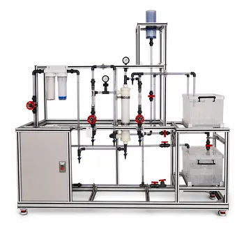
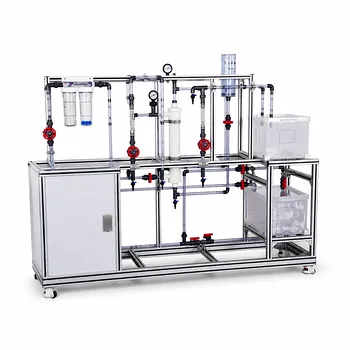
How To Demonstrate Membrane Selectivity Vs. Area Trade-Offs In Gas Dehydration Pilot Plants?

Here's how students can vividly demonstrate the trade-off between membrane selectivity and required area in a gas dehydration pilot plant.
By configuring a membrane test cell with a controlled water vapor/methane feed and a fixed dehydration target (e.g., -40°C dew point), students can measure the separation factor and compute the membrane area needed to achieve that target. When they compare results from membranes of different selectivity, they observe that a tenfold increase in selectivity—from 500 to 5000—reduces methane loss by only a few tenths of a percent, yet demands an 8‑fold larger membrane surface. This striking outcome teaches that maximum selectivity is rarely the optimal design choice when capital cost matters.

Core takeaway: In membrane gas dehydration, chasing the highest possible selectivity delivers only marginal improvement in product recovery while drastically inflating the required membrane area. The real lesson is about balancing performance with capital expenditure—a central trade-off in process engineering.

The Experimental Framework: How to Set Up the Demonstration

A well‑designed educational pilot plant can turn this trade-off into a tangible, data‑driven experience. The goal is to let students quantify how selectivity changes the membrane area needed to hit a specific dehydration target, holding other conditions constant.

Selecting the Model System

Start with a binary mixture that mimics industrial dehydration. Methane saturated with water vapor is ideal: it represents natural gas processing, is safe in a teaching lab, and provides a clear separation challenge. Set the feed pressure to a constant value—10 atm is typical for a small‑scale membrane dryer—and pre‑saturate the gas at a controlled temperature to maintain a known inlet humidity.

Defining the Separation Target

Give students a concrete performance goal, such as “produce dry gas with a dew point of −40 °C.” This fixed target forces them to calculate the required membrane area rather than simply observing a generic permeation rate. The inlet water concentration is known, so the mass balance yields the amount of water that must be removed per unit time.

Varying Selectivity Practically

In a pilot plant, selectivity isn’t a knob you turn—it’s a property of the membrane material. To demonstrate the trade-off, use:

Multiple membrane test cells loaded with commercial thin‑film composite membranes of different water/methane selectivities (e.g., 500, 1500, 5000).
Temperature variation on a single module: membrane selectivity often changes with temperature, allowing a single piece of hardware to generate multiple data points.
Simulation‑assisted experiments: collect real permeation data (flux, compositions) at one condition, then use membrane transport models (like Aspen Plus or custom Excel solvers) to extrapolate area requirements for higher hypothetical selectivities. This is especially powerful when physical membranes of extreme selectivity are unavailable.

Data Collection and Area Calculation

For each selectivity level, students measure:

Feed, retentate, and permeate flow rates.
Water concentration in each stream (via dew‑point meter or gas chromatography).
Membrane area already installed (the test cell’s active area).

They then calculate the separation factor α from the measured compositions:

α = (y_water / y_methane) / (x_water / x_methane)

where y is permeate mole fraction and x is feed mole fraction. The required total membrane area to meet the −40 °C dew‑point target is obtained by scaling the test cell area linearly with the water removal duty, accounting for the effective driving force (partial pressure difference) across the membrane. Because area is inversely proportional to water permeance, and high‑selectivity materials often exhibit significantly lower water permeance, the computed area escalates dramatically.

Visualizing the Trade-off: A Striking Result

When students plot “Methane loss” and “Required membrane area” against selectivity, the curve speaks volumes.

The Numbers That Hit Home

At 500 selectivity, with a pressure ratio of 80, the methane loss is around 3.2% and the membrane area is taken as a baseline. At 5000 selectivity, methane loss drops only to 2.75%—a negligible 0.45 percentage point improvement. Yet the membrane area must be increased by a factor of eight. These exact figures (from the primary reference) transform an abstract trade-off into a vivid “aha!” moment: the cost of that tiny purity gain is an 8× larger skid, more housing, and far greater capital outlay.

Connecting to Robeson’s Upper Bound

To deepen the lesson, have students overlay their data on a permeability–selectivity chart similar to Robeson’s upper bound. Supplementary references show that moving toward higher selectivity almost always means sacrificing permeance. This fundamental material constraint explains why area balloons—the water permeating flux drops so much that you need a huge surface just to move the same amount of water.

Understanding the Trade-offs: Capital vs. Operating Cost

The core pedagogical insight is not just the mathematical relationship; it’s the engineering economics.

The Cost of Over‑Specifying Selectivity

A membrane with 5000 selectivity might look superior on a spec sheet, but the 8‑fold area increase translates directly into more modules, larger vessels, and a heavier structural footprint. For a pilot‑plant exercise, students can estimate the module cost using catalog prices and see how the capital expenditure skyrockets. Meanwhile, the saved methane (from 3.2% down to 2.75% loss) has minimal revenue impact at typical natural gas prices, making the high‑selectivity option economically irrational.

The Role of Flux and Energy

Supplementary examples show that in air separation, a selectivity increase from 8 to 12 can cut compressor power by 29% while increasing area tenfold. In dehydration, the same pattern holds: if the goal is to minimize product loss, high selectivity is attractive only when membrane area is cheap and compression energy is expensive. In most pilot‑plant scenarios, the energy to re‑compress permeate or to maintain pressure is already fixed, so the area penalty dominates.

Avoiding a Common Pitfall: Mistaking Purity for Profitability

Students often assume that higher selectivity always means a better process. The pilot‑plant demonstration corrects this by showing that the thermodynamic benefit of higher selectivity saturates quickly in certain separations, especially when one component (water) is highly condensable and already permeates preferentially. Beyond a moderate selectivity, the marginal gain in retentate purity is minuscule, while the membrane cost escalates without bound.

Making the Right Choice for Your Goal

After the experiment, students should be able to make a reasoned selection.

If your primary focus is minimizing methane loss: Choose a moderately high selectivity, but only up to the point where the incremental recovery gain no longer justifies the extra membrane area. For the example shown, selectivities around 500–1000 strike a sweet spot.
If your primary focus is minimizing capital expenditure (membrane skid cost): Avoid jumping to the most selective membrane. A membrane with a separation factor near 500 will require far less area and will still yield a very dry product with acceptable hydrocarbon loss.
If your primary focus is energy efficiency in a multi‑stage configuration: Recognize that dehydration is often a pre‑treatment step. An overly selective membrane can create pressure‑drop and footprint issues that cascade through the process. Keep the dehydration module compact, and address final purity downstream.

The take‑home message is unambiguous: in membrane gas dehydration, the most selective material is rarely the most intelligent engineering choice—and a well‑designed pilot‑plant exercise lets students prove that to themselves, one data point at a time.

Summary Table:

Selectivity (Water/Methane)	Methane Loss (%)	Relative Membrane Area	Pedagogical Insight
500	3.20%	1.0x (Baseline)	Economically optimal; lower capital expenditure (CAPEX)
5000	2.75%	8.0x	Marginal recovery gain; highly inflated equipment footprint

Empower Your Students with Real-World Engineering Insights

LABPARK provides high-quality Educational and Vocational Unit Operations Pilot Plants in chemical engineering, bioprocess & biotech, and environmental & water treatment. Specially designed for universities, research institutes, and enterprises, our pilot plants allow students to actively demonstrate and calculate critical process trade-offs like membrane selectivity, flux, and area.

Ready to elevate your engineering lab? Contact LABPARK today to find the perfect pilot plant solution for your curriculum!