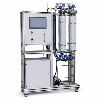
Temperature's impact on gas solubility is inverse and immediate. In any gas absorption unit operation, raising the solvent temperature lowers the equilibrium solubility of the gas in the liquid. This means absorption efficiency plummets at higher temperatures, while stripping (desorption) is favored. In a pilot plant setting, students can quantitatively verify this relationship by adjusting the solvent temperature with heat exchangers and measuring the resulting concentration changes across the column.
The core principle is simple: gas solubility decreases as temperature rises. By running a pilot plant at multiple controlled temperatures and analyzing both gas and liquid streams, students can calculate Henry’s law constants and directly map the solubility curve, turning an abstract thermodynamic rule into a tangible experimental result.
Why Temperature Drives Gas Solubility in Absorption
The Thermodynamic Foundation
Gas-liquid equilibrium is a delicate balance. As temperature increases, the kinetic energy of dissolved gas molecules rises, making it easier for them to overcome intermolecular forces and escape back into the gas phase. This directly lowers the gas solubility.
In practical terms, this means a cooler solvent can "hold" far more solute gas at the same partial pressure. The relationship is quantified through Henry’s Law: ( p = E \cdot x ), where the Henry’s coefficient ( E ) becomes larger as temperature rises, reflecting reduced solubility.
How This Shifts the Operating Regime
When you operate an absorption column with cold solvent, the driving force for mass transfer is maximized. You need less solvent flow and a shorter column to achieve the same removal. The opposite is true if the solvent is warm: the equilibrium line on a concentration diagram steepens, bringing the operating and equilibrium lines closer together and reducing the mass transfer driving force.
Observing the Effect Experimentally: A Student's Guide
The Pilot Plant Setup
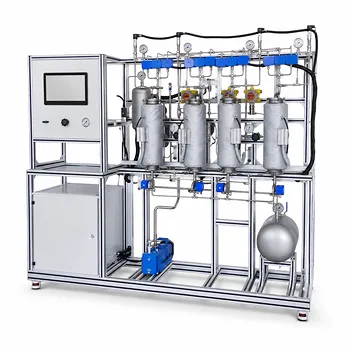
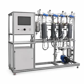
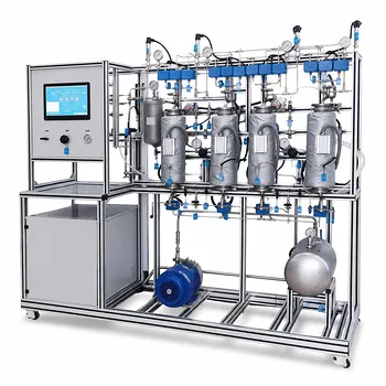
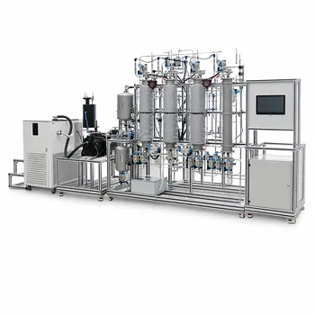
The key tool is a heat exchanger on the solvent inlet line. A typical educational pilot plant includes a temperature-controlled water bath or an electric heater/chiller linked to a shell-and-tube or plate heat exchanger. This lets students set a precise inlet solvent temperature. The column itself should be insulated and equipped with temperature sensors at the top and bottom.
The gas feed is kept steady in flow and composition. The liquid solvent, typically water for gases like CO₂, SO₂, or NH₃, enters at the top. Pressure regulators maintain a constant column pressure, isolating temperature as the only variable.
Measurement Protocol
To quantify the effect, follow this procedure:
- Set the solvent inlet to the lowest target temperature (e.g., 10°C) and stabilize the column.
- Measure the gas inlet and outlet concentrations—often with an online infrared gas analyzer or by periodic sampling.
- Measure the liquid outlet concentration—via titration, conductivity, or dissolved-gas sensors.
- Repeat the same steady-state measurement for multiple step-wise increases in temperature (e.g., 20°C, 30°C, 40°C), always allowing the column to reach equilibrium.
Calculating Henry’s Coefficient and Mapping the Curve
For each temperature, students can back-calculate the effective Henry’s coefficient ( E ) from the measured outlet liquid mole fraction and the known gas partial pressure at the column's bottom (using the gas outlet composition and total pressure). Plot ( E ) versus temperature to observe the exponential-like increase that thermodynamic models predict.
Alternatively, plot the absorption rate (mass of solute transferred from gas to liquid per unit time) against temperature. The curve will show a clear decline, confirming that temperature rise directly suppresses absorption.
Understanding the Trade-offs
The Diffusion Rate Tug-of-War
While low temperature boosts solubility, it has a counter-effect on molecular kinetics. The gas diffusion coefficient ( D ) is proportional to ( T^{3/2} ), meaning warmer conditions accelerate the movement of solute molecules through the solvent. This can speed up local mass transfer at the same driving force.
In a real column, this creates a trade-off: higher temperature boosts the mass transfer coefficient but slashes the driving force. The net effect is almost always negative for absorption: the solubility loss outweighs the diffusivity gain. For educational experiments, however, students may notice the outlet gas concentration changes slower than expected when moving from a very cold to a moderately cool temperature because the diffusivity improvement partially offsets the solubility loss.
The Coupling with Pressure
Temperature’s effect is amplified by the system pressure. Gas solubility increases with higher pressure. If students want to isolate the temperature effect, they must keep the column pressure absolutely constant. Even small pressure drifts can mask the temperature-induced solubility changes. A good practice is to fix the pressure at a value that keeps the process on the steep part of the solubility curve, making the temperature effect more dramatic.
Making the Right Choice for Your Student Experiment
- If your primary focus is demonstrating the thermodynamic principle: Prioritize running at three or four widely spaced temperatures (e.g., 10°C, 20°C, 35°C, 50°C) and measure the complete mass balance to compute Henry’s constants.
- If your primary focus is showing industrial absorption optimization: Operate at a constant, relatively low temperature and then spike the solvent temperature to observe how much absorption performance plunges—emphasizing why plants invest in cooling.
- If your primary focus is a combined heat and mass transfer study: Measure both gas outlet concentration and liquid outlet temperature rise to link the exothermic absorption heat effect with the solubility penalty, giving a more complete picture.
By transforming temperature from a textbook note into a dial on your pilot plant, you turn solubility theory into a measurable, memorable truth.
Summary Table:
| Parameter | Higher Temperature | Lower Temperature | Impact on Unit Operations |
|---|---|---|---|
| Gas Solubility | Decreases | Increases | Dominant driver of absorption efficiency |
| Henry's Constant (E) | Increases | Decreases | Determines equilibrium concentration |
| Diffusion Rate (D) | Increases | Decreases | Warmer temperatures speed up kinetics |
| Process Direction | Favors Stripping | Favors Absorption | Key to choosing operating parameters |
Elevate Your Chemical Engineering Lab with LABPARK
Bring thermodynamic theory to life with LABPARK's Educational and Vocational Unit Operations Pilot Plants. Specially designed for universities, research institutes, and enterprises, our advanced training systems for chemical engineering, bioprocess & biotech, and environmental & water treatment empower students to master gas absorption, heat transfer, and mass balance through hands-on practice.
Ready to upgrade your laboratory equipment? Contact LABPARK today to request a customized solution and quote for your institution.
Related Products
- Dual-Mode Gas Absorption and Desorption Unit Operations Training Pilot Plant
- Multi-Component Gas Pressure Swing Adsorption Pilot Plant for Unit Operations Education
- Carbon Dioxide Adsorption and Capture Educational Unit Operations Pilot Plant
- Packed Bed Absorption Educational Unit Operations Pilot Plant
- Absorption and Desorption Educational Unit Operations Pilot Plant
People Also Ask
- How do temperature and pressure affect gas absorption and desorption? Optimize Pilot Plant Performance
- How do two-film & penetration theories apply to gas absorption pilot plant teaching? Key pedagogical insights.
- How does partial pressure behavior influence gas absorption pilot plants? Master Mass Transfer
- How is the direction and driving force of mass transfer determined in a gas absorption unit operations pilot plant?
- What are the limitations of Henry's Law in gas absorption pilot plants? Avoid critical lab errors.