The relationship between fluid velocity and the convective heat transfer coefficient is immediately and quantitatively visible in a unit operations pilot plant. By using a heat exchanger with variable-speed pumps and precise instrumentation, the system allows you to physically manipulate flow and directly measure the thermal consequence. You are not just reading about the Dittus-Boelter correlation; you are generating the data that proves it, directly linking the physics of fluid motion to the rate of heat exchange.
A pilot plant demonstrates this relationship by allowing the deliberate, controlled variation of tube-side fluid velocity while measuring the resulting change in heat duty. This experiment directly reveals not only the fundamental $h \propto u^{0.8}$ power-law relationship in turbulent flow but also the critical transition from laminar to turbulent regimes, making an abstract equation a tangible, measurable reality.
The Core Mechanism: From Pump Speed to Heat Transfer
The demonstration hinges on a simple cause-and-effect chain. You change the pump speed, which changes the flow, which fundamentally alters the thermal boundary layer inside the tube.
Measuring the Direct Cause: Fluid Velocity
The pilot plant is instrumented to make the independent variable—velocity—perfectly clear. A variable speed pump or a control valve on the tube side lets you precisely alter the flow rate.
A dedicated flow meter provides a real-time reading of the volumetric flow rate ($V$). Since the tube's internal diameter ($d$) is known and fixed, the average fluid velocity ($u$) is calculated directly using the continuity equation. This gives you a precise value for the parameter you are controlling.
Calculating the Direct Effect: The Convective Coefficient
The dependent variable, the convective heat transfer coefficient ($h_i$), is revealed through a series of energy balance calculations. The pilot plant’s sensors provide the raw data necessary for this deduction.
First, you measure the inlet and outlet temperatures and the mass flow rate of both the tube-side and shell-side fluids. From these, you calculate the total heat duty ($Q$) transferred in the exchanger using $Q = \dot{m} c_p \Delta T$. This is the actual thermal energy moved.
Next, you calculate the log mean temperature difference (LMTD), which is the driving force for heat transfer. With the heat duty ($Q$), the known heat transfer area ($A$), and the LMTD known, you solve the fundamental equation $Q = U A \Delta T_m$ for the overall heat transfer coefficient ($U$). This value represents all thermal resistances combined.
Isolating the Tube-Side Resistance
The final experimental step is to isolate the tube-side coefficient ($h_i$) from the overall $U$ value. This makes the specific impact of velocity visible.
The pilot plant experiment often uses a modified Wilson plot technique or works from known, stable conditions. The overall resistance, $1/U$, is the sum of individual resistances: tube-side film ($1/h_i$), tube wall, and shell-side film ($1/h_o$), plus any fouling. By keeping the shell-side conditions absolutely constant while varying only the tube-side velocity, any change in the measured $1/U$ is solely attributable to the change in $1/h_i$. This experimental isolation provides a clear, empirical value for $h_i$ at each velocity setting.
Why the Pilot Plant Proves the $u^{0.8}$ Rule
Manipulating flow in the lab doesn't just generate numbers; it provides a visual and conceptual understanding of the governing physics. The pilot plant makes the mechanisms behind the equation intuitive.
Visualizing the Laminar Boundary Layer
The pilot plant experiment connects velocity directly to the concept of thermal resistance. In convective heat transfer, the dominant resistance is the stagnant, laminar sublayer that clings to the tube wall.
At low velocities, the flow may be laminar, and the boundary layer is thick. Heat must conduct through this thick, slow-moving film of fluid, acting like a blanket. When you increase the fluid velocity, you increase turbulence. The chaotic eddies in the turbulent core punch through this blanket, scrubbing the wall and drastically reducing the thickness of the laminar sublayer. The pilot plant data shows this as a sharp, non-linear increase in the $h_i$ coefficient as you transition to turbulent flow.
Validating the Power-Law Exponent
The specific exponent of 0.8 is a direct consequence of this turbulent mixing. The pilot plant provides the data to verify it precisely.
After calculating $h_i$ for several different turbulent flow velocities, a clear mathematical relationship emerges from a log-log plot of the data. The slope of the line correlating the Nusselt number to the Reynolds number will approximate 0.8, exactly as predicted by the Dittus-Boelter correlation. This experimental verification transforms a textbook exponent from an abstract number into a confirmed, observed physical fact. You can even observe the entrance effect, where the heat transfer coefficient is anomalously higher at the tube inlet because the boundary layer is initially much thinner.
Understanding the Trade-offs and Engineering Reality
An effective pilot plant demonstration does not end with the $u^{0.8}$ relationship. It is a perfect platform to introduce the critical, real-world constraints that transform a physics principle into an engineering decision.
The Inescapable Cost of Pumping Power
The most immediate trade-off is the relationship between velocity and pressure drop. While $h_i$ scales with velocity to the power of 0.8, the frictional pressure drop through the tube scales with velocity to the power of roughly 2.
By observing the pressure gauges on the pilot plant, you can see this dramatically. Doubling the velocity may improve heat transfer by about 74%, but it will increase the pressure drop by a factor of four. This means the pump's energy consumption skyrockets. The experiment teaches that maximizing heat transfer is never the sole objective; the real goal is an economically optimal balance between thermal performance and energy cost.
The Direct Impact on Fouling and Maintenance
A pilot plant can be used to demonstrate the inverse relationship between velocity and fouling. Operating with a fluid that has a mild fouling tendency clearly shows the effect.
At low velocities, dirt, scale, or biological matter deposits more readily on the heat transfer surface, creating a fouling resistance ($h_{id}$) that degrades performance over time. As you increase velocity, the higher shear stress at the wall physically scours the surface, reducing the rate of deposition. A pilot plant run over an extended period visualizes this perfectly, showing a stabilized $U$-value at high velocity and a continuously declining one at low velocity. This directly informs the heuristic of routing fouling-prone fluids through the tube side at a high velocity to enable easier cleaning and sustained performance.
Making the Right Choice for Your Goal
A unit operations pilot plant is a versatile tool, and the experiment’s focus can shift depending on the educational or research objective. The core data on velocity and heat transfer supports multiple levels of inquiry.
- If your primary focus is fundamental pedagogy: Run trials at a wide range of velocities, from laminar to fully turbulent. Calculate the Reynolds number, Nusselt number, and $h_i$ at each point. Plot the results to verify the 0.8 exponent and observe the dramatic change in heat transfer during the flow regime transition.
- If your primary focus is operational economics: Determine the optimum velocity. Measure both the heat transfer improvement and the associated pressure drop (energy cost) at each flow rate. Plot thermal duty and pumping power versus velocity on the same graph to find the economically justifiable operating range.
- If your primary focus is equipment longevity and reliability: Perform a long-duration run with a fouling-prone medium. Compare the decline in the overall heat transfer coefficient over time for a low-velocity case versus a high-velocity case to quantify the impact of shear stress on fouling mitigation.
By transforming abstract equations into a physical system you can touch and control, the pilot plant reveals that velocity is not just a variable in a formula, but the primary control lever for managing the delicate physics and economics of heat exchange.
Summary Table:
| Parameter | Key Relationship | Practical Engineering Impact |
|---|---|---|
| Fluid Velocity ($u$) | $u = V / A$ | Controlled variable changed via pump speed. |
| Convective Coefficient ($h_i$) | $h_i \propto u^{0.8}$ (Turbulent) | High velocity reduces boundary layer thickness, boosting heat transfer. |
| Pressure Drop ($\Delta P$) | $\Delta P \propto u^2$ | Higher velocities exponentially increase pumping energy costs. |
| Fouling Rate | Decreases as velocity increases | Wall shear stress scours scale and deposits, maintaining efficiency. |
Bring Thermal Physics to Life with LABPARK
Help your students and researchers bridge the gap between abstract equations and physical engineering. LABPARK provides state-of-the-art Educational and Vocational Unit Operations Pilot Plants in chemical engineering, bioprocess & biotech, and environmental & water treatment. Designed specifically for universities, research institutes, and enterprises, our pilot plants offer precise instrumentation to visualize and calculate real-world heat transfer and fluid dynamics.
Ready to upgrade your laboratory? Contact LABPARK today to discuss your custom pilot plant requirements!
Related Products
- Circulating Wind Tunnel Drying and Convective Heat Transfer Coefficient Determination Educational Pilot Plant
- Solid Spherical Heat Transfer Coefficient Determination Educational Chemical Engineering Pilot Plant
- Comprehensive Heat Transfer Coefficient Determination Educational Unit Operations Pilot Plant
- Shell and Tube Heat Exchanger Heat Transfer Coefficient Determination Educational Pilot Plant
- Three-Tube Heat Transfer Educational Pilot Plant for Unit Operations Training
People Also Ask
- Why transition from laminar to turbulent flow is critical in convective heat transfer pilot plants?
- How do tube arrangement & orientation affect condensation heat transfer? Optimize pilot plant performance.
- Why Are Thermal Properties Critical in Pilot Plants? Key Material Selection Factors
- What characterizes the transition to the falling rate drying period? Key scale-up insights.
- How are Nu, Re, and Pr used in forced convection pilot plants? Guide to Heat Transfer Scale-Up