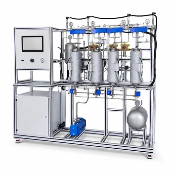
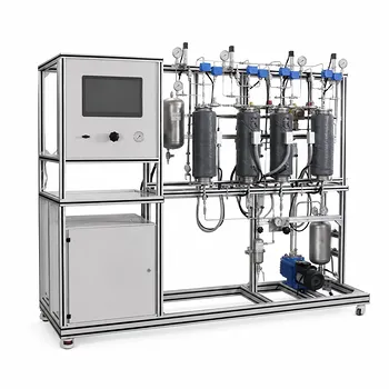
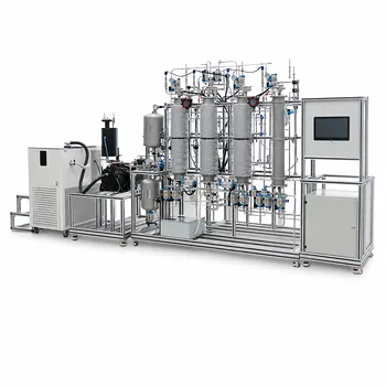
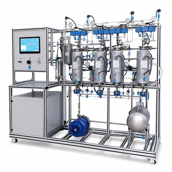
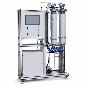
How To Measure Mass Transfer Coefficients Using Gas Absorption & Stripping Pilot Plants

Mass transfer coefficients are determined experimentally by measuring concentration changes and flow rates. In an educational gas absorption or stripping pilot plant, you bring a gas and liquid into counter-current contact inside a packed column, operate at steady state, and sample the solute concentration at the inlet and outlet of each phase. A material balance over the column gives the total absorption rate ((G_A)). You then calculate the log-mean driving force ((\Delta Y_m)) from the measured terminal concentrations and the equilibrium relationship, and finally apply (K_Y a = G_A / (V_p \cdot \Delta Y_m)) to obtain the volumetric overall mass transfer coefficient. For a deeper dive into individual film coefficients, students can determine the number of transfer units (NTU) and height of a transfer unit (HTU), then use variations of liquid and gas flow rates to separate liquid‑film and gas‑film resistances.

While the formula (K_Y a = G_A/(V_p \Delta Y_m)) provides a direct path to the overall volumetric coefficient, the true educational power of a pilot plant lies in dissecting the two‑film theory through HTU/NTU analysis, manipulating the liquid‑to‑gas ratio, and comparing physical with chemical absorption to reveal how each phase contributes to the total mass transfer limitation.

The Experimental Foundation: Measuring What Matters

Steady‑State Operation and Material Balances

Before any coefficient can be calculated, the column must operate at steady state. You fix the gas and liquid inlet flow rates and wait until outlet concentrations become constant—this ensures the solute mass entering the system balances the mass leaving. A simple material balance over the entire column for the solute yields the absorption rate ((G_A)) in moles per unit time. By measuring inlet and outlet solute mole fractions in the gas and liquid, and knowing the total molar flow rates, you can directly compute (G_A) from the difference between what enters and exits.

From Concentration Data to Driving Force

The mass transfer rate is proportional to a driving force, typically expressed as the difference between the actual gas‑phase mole fraction and the value that would be in equilibrium with the liquid at that point. Since concentrations change along the column, you use a log‑mean average driving force ((\Delta Y_m)). To compute (\Delta Y_m), you need the gas‑phase solute mole fractions at the bottom ((Y_1)) and top ((Y_2)), the corresponding equilibrium mole fractions ((Y^_1), (Y^_2)) obtained from Henry’s law or other equilibrium data, and the standard log‑mean formula. Pilot plants equipped with gas sensors and precise flow controllers make these measurements both straightforward and repeatable.

Calculating the Volumetric Coefficient (K_Y a)

Once (G_A) and (\Delta Y_m) are known, you determine the packed bed volume ((V_p)) from the column’s internal diameter and the height of the packing. The overall volumetric mass transfer coefficient is then (K_Y a = G_A / (V_p \cdot \Delta Y_m)). This single coefficient lumps the gas‑film resistance, the liquid‑film resistance, and the effective interfacial area ((a)) together. It is the fastest, most intuitive result you can extract—but it hides the microscopic story of which phase limits the process.

Deconstructing the Transfer Unit: HTU and NTU

Building the Operating Line and Equilibrium Curve

To separate film resistances, students move from the volumetric lumped coefficient to the transfer unit concept. You first construct an operating line by plotting the gas‑phase mole fraction against the liquid‑phase mole fraction at multiple points along the column—at minimum from the terminal measurements, but ideally using intermediate sampling taps. On the same diagram, draw the equilibrium curve based on Henry’s law for the solute‑solvent system. The slope of the operating line, (L_m/G_m) (the liquid‑to‑gas molar flow ratio), is a key lever you control by adjusting pump and valve settings.

Determining the Number of Transfer Units ((N_{OG}))

The number of transfer units represents the difficulty of the separation. Graphically, (N_{OG}) is the area between the operating line and the equilibrium curve, often calculated by numerical integration of (\int_{Y_2}^{Y_1} \frac{dY}{Y - Y^*}). You can also use the analytical expression based on the absorption factor (A = L_m/(m,G_m)) and the terminal concentrations, where (m) is the slope of the equilibrium line. In a teaching lab, performing this integration by hand—or with a simple spreadsheet—cements the relationship between thermodynamics, flow rates, and column performance.

Extracting Height of a Transfer Unit and Individual Coefficients

The total packed height ((Z)) is simply (Z = H_{OG} \times N_{OG}). Because (Z) is known from the pilot plant dimensions and (N_{OG}) is computed, you directly obtain the overall height of a transfer unit ((H_{OG})). The relationship (H_{OG} = H_G + \frac{m,G_m}{L_m} H_L) then links (H_{OG}) to the individual gas‑film ((H_G)) and liquid‑film ((H_L)) heights. By running experiments at several (L_m/G_m) ratios and plotting (H_{OG}) against (m,G_m/L_m), the intercept yields (H_G) and the slope yields (H_L)—a classic technique that reveals which film dominates the resistance.

Beyond the Overall Coefficient: Probing Film Resistances

Using Chemical Absorption to Isolate Liquid‑Film Resistance

When you switch from physical absorption (e.g., CO₂ in water) to chemical absorption (e.g., CO₂ in an amine or alkaline solution), the liquid‑phase resistance can be dramatically reduced. A fast chemical reaction consumes the dissolved solute within the liquid film, effectively making (H_L) negligible. Under these conditions, the measured (H_{OG}) approximates (H_G) alone, allowing you to estimate the gas‑film coefficient directly. Comparing results from physical and chemical systems teaches a fundamental design principle: selecting a reactive solvent can shift the controlling resistance and drastically shrink column height.

Correlations and Effective Interfacial Area

A pilot plant also lets you validate empirical correlations, such as the widely cited Onda correlations for (k_L) and effective interfacial area (a_e). By measuring the pressure drop and liquid holdup across different packing types (e.g., ceramic rings vs. high‑porosity plastic packings), you can back‑calculate the effective wetted area. Students see that not all geometric surface area is active—channeling, wetting, and loading phenomena all influence (a_e), and those correlations carry an element of uncertainty that hands‑on data can illuminate.

Understanding the Trade‑offs

Every educational experiment involves compromises between accuracy, safety, and conceptual clarity. Recognizing these trade‑offs is essential for interpreting your pilot plant data correctly.

Flooding, Loading, and Operational Limits

As you increase gas and liquid flow rates to explore mass transfer behavior, you will eventually encounter loading and then flooding. Near flooding, liquid holdup rises sharply, pressure drop spikes, and mass transfer efficiency may actually decrease. Your data becomes unreliable if you unknowingly operate in the flooding region; students must learn to identify the classic pressure‑drop curve and stay within the stable region for valid coefficients.

Physical vs. Chemical Systems: Precision vs. Safety

Physical systems like CO₂‑water are safe and straightforward, but the liquid‑film resistance is often high, making (H_{OG}) large and changes in (H_G) harder to detect. Chemical systems like CO₂‑amine offer larger driving forces and smaller columns, but they introduce heat effects, solvent degradation, and safety concerns that can complicate data analysis. The choice of system determines which mass transfer phenomenon you can best isolate—and what level of experimental rigor you must apply.

Packing Type and Its Impact on Data Validity

High‑performance structured packings may give excellent efficiency but obscure the link to classic correlations taught in lectures. Using classic random packings (Raschig rings, Berl saddles) aligns your data with textbook Onda correlations, but you must account for older packing factors. The pilot plant’s interchangeable packing bed allows you to test both, turning a potential confusion into a lesson in model applicability.

The Assumption of Steady‑State and Isothermal Conditions

All the straightforward analysis methods assume steady state and negligible temperature change. In a teaching lab, absorption of CO₂ by an amine solution can release heat, bending the equilibrium line and violating the isothermal assumption. Students must check whether their temperature profiles are flat; if not, more advanced non‑isothermal correction methods become a valuable next step.

Making the Right Choice for Your Educational Goal

The pilot plant is a flexible tool, and the experimental plan should match the learning objective. Here is how to tailor your approach.

If your primary focus is generating a quick, reliable overall coefficient: Use physical absorption, maintain steady liquid and gas flow rates well below flooding, measure terminal concentrations, and apply the log‑mean driving force method to obtain (K_Y a).
If your primary focus is understanding the two‑film theory and individual film coefficients: Run multiple experiments at different (L_m/G_m) ratios, determine (H_{OG}) and (N_{OG}) for each, then extract (H_G) and (H_L) from the (H_{OG}) vs. (mG_m/L_m) plot.
If your primary focus is experiencing the impact of packing and hydrodynamics: Measure pressure drop and holdup curves for at least two packing types, observe loading and flooding visually, and discuss how these phenomena affect (a_e) and the valid operating window.
If your primary focus is validating design correlations: Collect data over a range of flow rates for a known packing, compute experimental (k_L) and (a_e), and compare them directly to the Onda predictions, noting the scatter and systematic deviations.

Hands‑on operation of a gas absorption pilot plant transforms mass transfer from an abstract set of differential equations into a tangible, measurable reality—once you understand what to measure, how to reduce it, and what limitations your experimental choices introduce.

Summary Table:

Experimental Focus	Key Parameters Measured	Primary Calculation Method
Overall Volumetric Coefficient ($K_Y a$)	Inlet/outlet concentrations, gas/liquid flow rates	$K_Y a = G_A / (V_p \cdot \Delta Y_m)$ (Log-Mean Driving Force)
Individual Film Resistances ($H_G$, $H_L$)	Overall HTU ($H_{OG}$) at varying $L_m/G_m$ ratios	Graphical slope/intercept of $H_{OG}$ vs. $m G_m / L_m$
Hydrodynamics & Wetted Area	Pressure drop, liquid holdup across packing types	Validation via Onda correlations and flooding limit curves

Elevate Your Chemical Engineering Lab with LABPARK

Ready to bring complex mass transfer theory to life? LABPARK designs and delivers advanced Educational and Vocational Unit Operations Pilot Plants tailored for chemical engineering, bioprocess & biotech, and environmental & water treatment programs.

We provide universities, research institutes, and enterprises with robust, safe, and highly accurate systems that bridge the gap between textbook equations and hands-on industrial reality.

Contact LABPARK today to discover how our pilot plants can enhance your laboratory's capabilities!