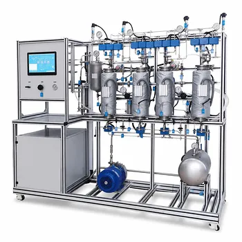
Why Are Liquid-Phase Mass Transfer Rates In Pilot Plants Comparable To Gas-Phase Rates? Key Insights

Liquid-phase diffusion coefficients are five orders of magnitude smaller than those in gases—yet, in absorption pilot plants, the mass transfer rates can be surprisingly similar. This apparent contradiction resolves when you look beyond the diffusion coefficient alone: mass transfer flux is the product of the diffusion coefficient and the concentration driving force. Liquids possess an enormously higher molar density than gases, which amplifies even a modest concentration difference into a steep molar concentration gradient. Under the steady-state conditions typical of a gas absorption pilot plant, this steeper driving force offsets the slower molecular movement, allowing liquid-phase mass transfer rates to reach the same order of magnitude as those in the gas phase.

The liquid phase compensates for its intrinsically slow molecular diffusion by operating with much steeper concentration gradients, made possible by the high molar density of liquids. In gas absorption pilot plants, this means the overall mass transfer rate is driven by a balance between the diffusion coefficient and the size of the driving force, not just the coefficient alone.

Understanding the Driving Force Behind Mass Transfer

The mass transfer rate is not a single number—it’s a product of two components. To see why liquid and gas phases can deliver comparable transfer rates, you have to examine each component’s contribution.

Fick’s First Law and the Concentration Gradient

Fick’s first law states that the diffusive flux ( J ) (the transfer rate per unit area) equals the diffusion coefficient ( D ) multiplied by the concentration gradient ( \Delta C / \Delta x ).

In gases, the diffusion coefficient is large but the molar concentration of a solute can be very low. For example, a typical gas stream with a few percent of the absorbed species might have a bulk concentration of only a few mol/m³.
In liquids, the molar concentration of the solvent itself is enormous (water is ~55,000 mol/m³). Even a small difference in solute mole fraction translates into an extremely large molar concentration gradient.

This means the driving force term (( \Delta C )) in liquids can be thousands of times larger than in gases, directly offsetting the five-order-of-magnitude deficit in ( D ).

Diffusion Coefficient vs. Concentration Gradient: The Balancing Act

It’s the multiplication that matters.

Typical gas-phase diffusion coefficient: ( 10^{-5} , \text{m}^2/\text{s} )
Typical liquid-phase diffusion coefficient: ( 10^{-9} , \text{m}^2/\text{s} )

If the liquid-phase concentration gradient is ( 10^4 ) times steeper than the gas-phase gradient, the resulting flux becomes comparable. In many absorption columns, the liquid enters relatively solute‑free and leaves partially saturated, sustaining a large average driving force over the entire column height.

Steady‑state operation locks in this balance. The column reaches an equilibrium where the flux through the gas film equals the flux through the liquid film. Because the liquid can sustain a much larger gradient, its “slower” molecules end up delivering a similar amount of solute per unit area.

Why Liquids Can Sustain Such Steep Concentration Gradients

The high molar density is the hardware; the operating conditions in a pilot plant provide the environment that exploits it.

Molar Density as an Amplifier

A liquid’s molar density acts like a concentration multiplier.

At 1 atm and 25°C, air has a molar density of about 40 mol/m³. A 1% (mol) CO₂ stream yields a bulk CO₂ concentration of ~0.4 mol/m³.
Liquid water, at the same temperature, has a molar density of 55,500 mol/m³. Even if the dissolved CO₂ concentration difference is only 0.1% on a mole fraction basis, that’s a 55.5 mol/m³ difference—more than a hundred times larger than the gas-phase driving force for the same mole fraction change.

This inherent amplification means that the liquid phase does not need to rely solely on molecular mobility; it uses its enormous “concentration reserve” to push solute across the interface.

Steady-State Column Operation Maintains the Advantage

In a counter‑current absorption pilot plant, the gas and liquid flow in opposite directions, keeping the overall driving force high along the entire column.

The gas phase continually contacts fresh solvent at the bottom, maintaining a favorable concentration difference for absorption.
The liquid phase remains far from equilibrium with the gas at most points, preventing the gradient from collapsing.

This steady‑state dynamic means the liquid-phase concentration gradient never relaxes to the low values that would cripple its flux. The column is deliberately designed and operated to hold the liquid in a state where its high‑concentration phenotype translates into high transfer rates.

Understanding the Trade‑offs

The fact that liquid-phase rates can match gas-phase rates does not mean the liquid resistance is always negligible. Several practical factors can shift the balance.

When the Liquid Phase Can Still Be the Bottleneck

High solvent viscosity: Increases resistance to molecular movement, reducing the effective liquid‑side mass transfer coefficient. In pilot plants, viscous solvents like certain amines or ionic liquids can make liquid‑film resistance dominant despite the steep gradient.
Low temperature or near‑equilibrium operation: A shallower concentration gradient directly reduces the flux. If the liquid leaves the column close to equilibrium with the inlet gas, the driving force collapses.
Nonisothermal effects: Fast absorption of a highly soluble gas or a chemical reaction releases heat at the interface, locally raising the temperature. This reduces the gas solubility (Henry’s law constant increases), shrinking the effective concentration gradient. The result is a lower absorption flux than isothermal models predict.
Absorption parameter imbalance: The ratio ( m G_m / L_m ) influences which phase controls the overall transfer. An overly low solvent flow rate (( L_m )) makes the operating line approach the equilibrium line, concentrating the resistance in the liquid film. Optimal pilot‑plant operation targets ( m G_m / L_m ) between 0.7 and 0.8 to balance the resistances.

Why These Limitations Matter for Pilot Plants

Pilot‑scale experiments let you actively probe these trade‑offs. By changing liquid flow rates, you alter the slope of the operating line and can visually see how the number of transfer units (NTU) changes. By measuring the temperature profile, you can detect the onset of interfacial heating and correct scale‑up assumptions.

Ignoring the interplay between diffusion coefficient, concentration gradient, and temperature can lead to overestimating the efficiency of a full‑scale column if the pilot data are treated under simplistic isothermal assumptions.

How to Apply This to Your Pilot Plant or Design Project

Understanding why liquid-phase rates can be high lets you make deliberate choices about solvents, operating conditions, and interpretation of experimental data.

If your primary focus is maximizing absorption efficiency: Choose solvents with high solute capacity (to sustain a steep concentration gradient) and manage viscosity through temperature control. Adjust the liquid‑to‑gas ratio to keep the operating line far from equilibrium.
If your primary focus is accurate scale‑up: Do not rely on isothermal models without checking interfacial temperature rise. Pilot‑plant experiments with fast reactions should explicitly measure the temperature jump or use coupled energy‑mass balance models (e.g., penetration or film theory) to avoid overpredicting the flux.
If your primary focus is determining the rate‑limiting step: Vary the liquid flow rate (to alter the liquid‑side coefficient) and the gas flow rate (to alter the gas‑side coefficient) independently while measuring the overall mass transfer coefficient. If the overall coefficient changes strongly with liquid flow, the liquid film is controlling.
If your primary focus is educational demonstration: Leverage the fact that liquid‑phase concentration gradients can be directly visualized via color‑change indicators in pilot‑scale absorption columns to give students an intuitive grasp of how the driving force offsets the low diffusion coefficient.

An absorption pilot plant is not just a smaller version of an industrial unit—it’s a laboratory for understanding the physical dance between diffusion coefficients and concentration gradients. The liquid phase punches above its molecular weight precisely because it stores so much solute in a small volume, and steady‑state operation keeps that potential fully engaged.

Summary Table:

Parameter	Gas Phase	Liquid Phase
Diffusion Coefficient ($D$)	High ($\sim 10^{-5} \text{ m}^2/\text{s}$)	Low ($\sim 10^{-9} \text{ m}^2/\text{s}$)
Molar Density	Low ($\sim 40 \text{ mol/m}^3$)	Very High ($\sim 55,500 \text{ mol/m}^3$ for water)
Concentration Gradient ($\Delta C$)	Shallow / Low	Steep / High (amplified by molar density)
Mass Transfer Driver	High molecular mobility	Large concentration driving force

Optimize Your Chemical Engineering Lab with LABPARK

To master complex concepts like mass transfer rates, hands-on learning is essential. LABPARK designs and manufactures high-quality Educational and Vocational Unit Operations Pilot Plants specializing in chemical engineering, bioprocess & biotech, and environmental & water treatment.

We help universities, research institutes, and enterprises equip their facilities with robust, industry-scale teaching tools that bridge the gap between theoretical physics and practical application.

Ready to elevate your engineering curriculum or research capabilities? Contact LABPARK today to discuss your customized pilot plant requirements!