How Do Electrolytes Affect Phase Equilibrium In Absorption Pilot Plants, And How To Calculate It?

Electrolytes reduce the physical solubility of gases like carbon dioxide in aqueous solutions—a phenomenon called the “salting-out” effect. In an absorption pilot plant, this means that for the same partial pressure of CO₂, the equilibrium concentration in a salt-loaded solvent will be lower than in pure water. Quantifying this change is essential for accurate mass‑transfer calculations, and it is done by relating the Henry’s law constant (or distribution coefficient) in the electrolyte solution to the solution’s ionic strength through empirical salting‑out coefficients.

The core challenge: electrolytes push the equilibrium away from the liquid side, making the gas harder to absorb. Engineers capture this shift with relationships like the van Krevelen‑Hoftijzer equation ( \log_{10}(H / H_0) = h I ) or an extended form ( \ln(m_i / m_{i0}) = b I + b' c_i ), where (I) is the ionic strength and (h, b, b') are ion‑ and gas‑specific constants. The right approach depends on the solution complexity and the level of accuracy required for your pilot‑scale model.

The Salting‑Out Effect: Why Electrolytes Change the Equilibrium

When salts (electrolytes) dissolve in water, they do more than just change the solution’s conductivity. They alter the thermodynamic activity of the solvent and the dissolved gas, directly impacting phase equilibrium.

How Ions Compete with Gas Molecules

The water molecules that would normally solvate CO₂ are instead tightly bound in hydration shells around the cations and anions. This leaves fewer “free” water molecules to interact with the gas, so the gas is effectively squeezed out of the liquid phase.

The Role of Ionic Strength as a Master Parameter

The extent of salting‑out is not directly proportional to the mass of salt added. It scales with the ionic strength (( I )) of the solution:

[ I = \frac{1}{2} \sum c_i z_i^2 ]

where ( c_i ) is the concentration of each ion and ( z_i ) is its charge. Even chemically different salts produce similar salting‑out effects if they generate the same ionic strength, provided their individual ion interactions are similar.

Quantifying the Change: From Ionic Strength to a Corrected Henry’s Constant

Your pilot‑plant data almost certainly rely on Henry’s law to connect gas‑phase partial pressure and liquid‑phase concentration. Electrolytes effectively increase the Henry’s constant ((H))—you need a larger partial pressure to dissolve the same amount of gas.

The van Krevelen‑Hoftijzer Equation – The Workhorse Method

The most widely used empirical correction for pilot‑plant and industrial modelling is:

[ \log_{10}\left(\frac{H}{H_0}\right) = h \cdot I ]

( H ) = Henry’s constant in the electrolyte solution
( H_0 ) = Henry’s constant in pure water (at the same temperature)
( I ) = ionic strength of the solution
( h ) = the salting‑out coefficient, which sums contributions from the gas and all ions present:

[ h = h_g + h_+ + h_- ]

Published tables give (h) values for common ions (Na⁺, Cl⁻, CO₃²⁻, etc.) and gases. You simply add them up based on your solvent composition, compute (I), and get the corrected (H) in seconds.

When the Gas Concentration Itself Becomes Important

The primary reference highlights a slightly more detailed relationship that acknowledges the dissolved gas concentration ((c_i)):

[ \ln\left(\frac{m_i}{m_{i0}}\right) = b I + b' c_i ]

Here, (m_i) and (m_{i0}) are the distribution (partition) coefficients in the electrolyte solution and in pure water, respectively. The (b' c_i) term becomes significant only for very soluble gases or when the pilot plant operates at elevated pressures where (c_i) is no longer negligible. For dilute CO₂ in moderately alkaline or amine‑based solutions, (b' c_i) is often dropped, and the equation collapses to a form similar to van Krevelen‑Hoftijzer when ( \ln(m_i/m_{i0}) \approx 2.303 \log_{10}(H/H_0) ).

Step‑by‑Step for Your Pilot Plant Experiment

Measure or calculate the electrolyte composition (e.g., Na⁺, Cl⁻, CO₃²⁻ from amine degradation products or added salts).
Compute ionic strength (I) from all ions present.
Look up the salting‑out coefficient (h)
- Combine tabulated values for the gas (CO₂ (h_g)) and for each ion (e.g., (h_{Na^+}), (h_{Cl^-})).
- If using the primary reference’s approach and relevant ion‑specific correction factors (like (k_s, k^+, k^-) for low H⁺ concentrations), apply those in place of the simpler summation.
Correct the pure‑water Henry’s constant to obtain (H) at your solution conditions.
Apply the corrected Henry’s law in your equilibrium calculations. For purely physical absorption, that means (p_{CO_2} = H \cdot x_{CO_2}). For chemically reactive systems, the corrected physical Henry’s constant still serves as the basis onto which the chemical enhancement factor is applied.

Trade‑offs, Limitations, and Common Pitfalls

Empirical coefficients are not universal. The (h) values were typically determined for single‑salt systems. In complex electrolyte mixtures (e.g., loaded amine solutions with multiple cations and anions), the simple additivity rule may over‑ or under‑estimate the salting‑out effect. Cross‑ion interactions can cause deviations that reach 10–15 %.

The ionic strength correction alone ignores chemical consumption. In a pilot plant running chemical absorption (e.g., amine scrubbing of CO₂), the equilibrium partial pressure is drastically reduced by the reaction. However, the physical solubility behind that reaction is still governed by the electrolyte‑corrected Henry’s constant. Failing to correct for salting‑out will bias your kinetic and capacity calculations, especially in lean or heat‑stable salt‑loaded solutions.

High‑charge‑density ions dominate. Ions like CO₃²⁻ or SO₄²‑ contribute disproportionately to ionic strength (because of (z_i^2)) and to the salting‑out coefficient. Small measurement errors in their concentration propagate quickly. Double‑check your solution analysis and consider using activity‑coefficient models (e.g., Pitzer) if precision is mission‑critical.

Temperature dependency is separate. The relations discussed here correct for ionic effects at a given temperature. You must still account for the intrinsic temperature dependence of (H_0) using a van’t Hoff‑type relationship.

Making the Right Choice for Your Pilot‑Plant Modelling

Your decision on which calculation method to adopt depends on what you are trying to achieve and the level of complexity you can manage in your data processing.

If your primary focus is fast screening of saline solvents or waste‑water streams: Use the van Krevelen‑Hoftijzer method with tabulated ion contributions. It is quick, transparent, and sufficient for most engineering accuracy needs.
If your pilot plant handles very high electrolyte concentrations (I > 3 mol L⁻¹) or high‑pressure CO₂: Adopt the extended (\ln(m_i/m_{i0})) form with (b' c_i) or switch to a full electrolyte activity coefficient model. This avoids systematic under‑prediction of the liquid‑phase capacity.
If the goal is to decouple physical and chemical effects in a reactive absorption column: First compute the salting‑out‑corrected Henry’s constant. Then overlay the chemical enhancement from the reaction equilibrium. This gives you a clean, modular framework for diagnosing whether an efficiency drop comes from the electrolyte matrix or from a loss of chemical reactivity.

Ultimately, the presence of electrolytes is not a minor correction—it can shift the equilibrium line enough to change the required column height. By embedding a simple ionic strength dependency into your data analysis, you turn the pilot plant from a “black box” into a predictive tool.

Summary Table:

Method	Key Equation	Ideal Application	Major Advantage
van Krevelen‑Hoftijzer	$\log_{10}(H / H_0) = h I$	Fast screening of saline solvents & low-to-moderate concentrations	Simple, relies on widely available tabulated ion constants
Extended Equation	$\ln(m_i / m_{i0}) = b I + b' c_i$	High-pressure CO₂ capture or high electrolyte concentrations ($I > 3\text{ mol L}^{-1}$)	Accounts for dissolved gas concentration to prevent systematic errors
Electrolyte Models (Pitzer)	Activity coefficient calculations	Precision-critical thermodynamic modeling & complex mixtures	High accuracy; accounts for multi-ion interactions

Optimize Your Chemical Engineering Labs with LABPARK

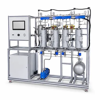
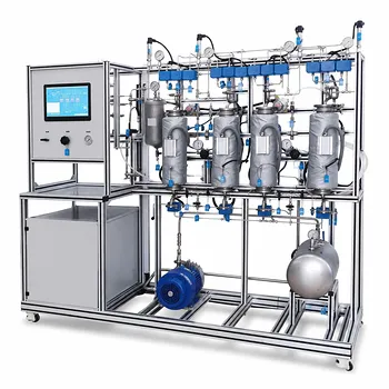
Accurate thermodynamic modeling is only half the battle—having the right physical infrastructure is key to validating your research. LABPARK provides state-of-the-art Educational and Vocational Unit Operations Pilot Plants in chemical engineering, bioprocess & biotech, and environmental & water treatment tailored for universities, research institutes, and enterprises.

Whether you are researching carbon capture, gas absorption, or advanced separation processes, our pilot plants deliver the reliability and scalability your project demands.

Contact LABPARK today to discuss your laboratory requirements and get a customized solution!