Electrolytes in a solvent almost always reduce gas solubility—a phenomenon known as the salting‑out effect. This decrease in the solvent's capacity to hold dissolved gas is not a trivial nuance; it can fundamentally alter the performance of a chemical or environmental engineering pilot plant. Quantitatively, operators track this shift using the van Krevelen and Hoftijzer equation, which relates the change in Henry’s law constant to the solution’s ionic strength and a specific salting coefficient.
Core Takeaway: The salting‑out effect directly diminishes gas solubility, shifting the gas‑liquid equilibrium and the driving force for mass transfer. In absorption pilot plants, this is rigorously quantified using the van Krevelen and Hoftijzer equation, allowing engineers to compensate for ionic strength and accurately predict column performance when scaling up processes involving saline streams.
The Salting‑Out Effect: Why Salts Drive Gas Out of Solution
Electrolytes alter the very structure of water, weakening its ability to surround and hold gas molecules.
Electrostatic Tightening of the Solvent
Dissolved ions (e.g., Na⁺, Cl⁻, Ca²⁺, SO₄²⁻) exert strong electrostatic fields. These fields pull water molecules into tight hydration shells, which reduces the “free” water available to solvate neutral gas species.
The result is a reduction in the effective solvent volume for the gas. This drives the gas out of solution and into the vapor phase—the classic salting‑out effect.
The Practical Consequence for Pilot Plants
When a saline wastewater or an industrial brine is used as the scrubbing liquid in an absorption column, the equilibrium curve shifts. For a given partial pressure, the liquid‑phase concentration of the target gas (e.g., oxygen for stripping or CO₂ for capture) will be lower than predicted by pure‑water data.
Without correction, the pilot plant data cannot be reliably scaled up.
Quantifying the Shift: The van Krevelen‑Hoftijzer Equation
The gold‑standard tool for quantifying salting‑out in gas‑liquid systems is the empirical equation developed by van Krevelen and Hoftijzer.
The Core Equation
The relationship is expressed as:
log₁₀(H/HB) = h · I
Here, H is Henry’s constant in the electrolyte solution, and HB is Henry’s constant in pure water. I is the ionic strength (mol/L), a measure of the total ion concentration and charge. The term h is the overall salting coefficient.
An increase in H (H > HB) means the gas is less soluble. The equation therefore directly translates ionic strength into a quantifiable solubility penalty.
Breaking Down the Salting Coefficient (h)
The term h is not a mystery constant—it is the additive sum of contributions from the gas and the specific ions present:
h = hg + h⁺ + h⁻
- hg: Contribution from the gas species.
- h⁺: Contribution from the cation (e.g., Na⁺).
- h⁻: Contribution from the anion (e.g., Cl⁻).
These individual coefficients are experimentally determined and widely tabulated. By looking up the values for the gas and the salt being used, a pilot plant operator can calculate h and, with the measured ionic strength, immediately correct the solubility.
Practical Application in an Absorption Pilot Plant
Knowing the theory is only half the battle—the real value lies in applying it during plant operation to obtain rigorous mass transfer data.
A Step‑by‑Step Quantification Process
In operation, a researcher or engineer follows a clear workflow:
- Analyze the liquid phase: Measure the concentration of all ionic species in the solvent to calculate the ionic strength (I).
- Identify the system components: Determine the target gas and the dominant salt in the solution.
- Look up the coefficients: Obtain hg, h⁺, and h⁻ from reference tables to compute the overall h.
- Calculate the corrected Henry’s constant: Use the equation to find H for the saline solvent at the operating temperature.
- Apply the corrected equilibrium: Use the new H in place of the pure‑water value when plotting the equilibrium line and calculating the driving force.
Many educational and research pilot plants also make use of ion‑specific empirical correction factors (k_s, k⁺, k⁻) that adjust the equilibrium constant directly when hydrogen ion concentration is low. While the form differs from the van Krevelen‑Hoftijzer equation, the principle is identical: use the solution’s ionic composition to refine the equilibrium prediction.
Impact on Pilot Plant Operation: From Equilibrium to Mass Transfer Efficiency
The corrected solubility does more than shift a line on a graph—it can change how you operate the column.
For a highly soluble gas that is normally gas‑film controlled: A strong salting‑out effect can push the equilibrium constant H much higher, effectively making the gas less soluble. This can shift a significant portion of the mass transfer resistance into the liquid film, meaning that purely increasing gas turbulence will no longer give a proportional increase in absorption rate.
In a pilot plant, this dictates a change in operational strategy. Operators must now focus on optimizing liquid distribution and packing wettability to enhance the liquid‑side mass transfer coefficient, rather than just the gas velocity.
Understanding the Trade‑offs and Limitations
No empirical correction is perfect, and applying the salting‑out equation blindly can lead to errors.
Accuracy Boundaries of the van Krevelen‑Hoftijzer Equation
The equation is most reliable at moderate ionic strengths typical of many process streams. At very high salt concentrations, the linear relationship with ionic strength can break down and require higher‑order terms or entirely different models (like the Pitzer model).
The coefficients h are also temperature‑dependent. A set of coefficients valid at 25°C will introduce error if the pilot plant is operated at 10°C or 60°C without the proper temperature correction.
The Assumption of a Single Salt System
The additive model (h = hg + h⁺ + h⁻) works beautifully for a single, fully dissociated salt. In real multi‑electrolyte brines, ion‑pair interactions can create non‑ideal behavior, making the simple summation less accurate.
Pilot plant operators must validate the predicted H with a direct sample analysis whenever the solvent is a complex mixture of unknown or industrial origin.
Making the Right Choice for Your Pilot Plant Goal
How you integrate the salting‑out quantification depends on the objective of your pilot‑scale study.
- If your primary focus is scaling up an industrial process with saline wastewater: Incorporate the van Krevelen‑Hoftijzer correction directly into your material balance model. Using pure‑water solubility data will underestimate the required liquid flow rate and lead to a failing full‑scale design.
- If your primary focus is teaching core absorption principles with a simple system: Deliberately add a known salt (like NaCl) to the water tank to demonstrate the salting‑out effect. Use the equation to let students predict the shift in the equilibrium line before they measure it, reinforcing the thermodynamic fundamentals.
- If your primary focus is maximizing mass transfer efficiency in a given column: Use the corrected H to re‑evaluate whether the controlling resistance has shifted. If the salt content moves the system toward liquid‑film control, redirect your optimization efforts toward liquid distribution and packing selection.
A rigorous, equation‑driven respect for the salting‑out effect transforms pilot plant operation from a source of puzzling data into a precise, scalable predictor of real‑world separation performance.
Summary Table:
| Concept / Parameter | Description & Formula | Impact on Pilot Plant Operation |
|---|---|---|
| Salting-Out Effect | Dissolved ions compress solvent structure, reducing gas solubility | Shifts the gas-liquid equilibrium curve; lowers absorption driving force. |
| Quantification Equation | $\log_{10}(H/H_B) = h \cdot I$ | Computes corrected Henry's constant ($H$) to prevent underestimating equipment size. |
| Salting Coefficient ($h$) | Additive sum of gas and ion constants: $h = h_g + h^+ + h^-$ | Allows operators to calculate exact solubility shifts for complex saline streams. |
| Mass Transfer Control | Higher ionic strength shifts resistance to the liquid film | Requires optimization of liquid distribution and packing instead of gas velocity. |
Advance Your Chemical & Environmental Engineering Research with LABPARK
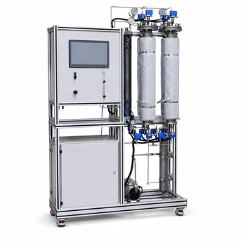
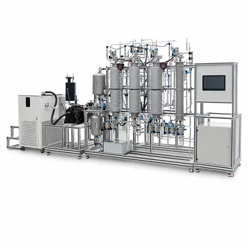
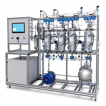
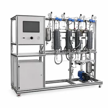
Accurately analyzing mass transfer and thermodynamic properties requires reliable, industry-grade testing systems. LABPARK provides state-of-the-art Educational and Vocational Unit Operations Pilot Plants in chemical engineering, bioprocess & biotech, and environmental & water treatment.
Tailored for universities, research institutes, and enterprises, our pilot systems deliver:
- Precise Process Control: Real-world simulation of absorption, stripping, and extraction.
- Scalable Data Acquisition: Reliable measurements to model complex electrolyte systems accurately.
- Robust Educational Value: Practical, hands-on training platforms for the next generation of engineers.
Transform your research and training capabilities today—contact our technical experts now to discuss your custom pilot plant configuration.
Related Products
- Carbon Dioxide Absorption and Desorption Educational Pilot Plant for Carbon Capture Studies
- Absorption and Desorption Educational Unit Operations Pilot Plant
- Packed Bed Absorption Educational Unit Operations Pilot Plant
- Multimodal Absorption and Desorption Pilot Plant for Unit Operations Training
- Dual-Mode Gas Absorption and Desorption Unit Operations Training Pilot Plant
People Also Ask
- How does operating pressure influence the transition between absorption and desorption in a CO2 pilot plant?
- How do temperature and pressure affect gas absorption and desorption? Optimize Pilot Plant Performance
- How do temperature variations affect CO2 transport models in pilot plants? Model vs Reality
- How is the number of transfer units (N_OL) calculated and verified? Master Desorption Mass Transfer
- What unit operations are critical for CCUS training pilot plants? Build hands-on engineering expertise.