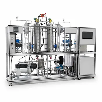
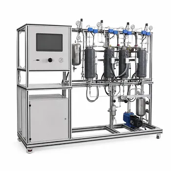
What Process Parameters And Material Balance Principles Govern The Evaluation Of Membrane Gas Separation Pilot Plants?

Membrane gas separation pilot plants are evaluated by combining operating data with steady-state component balances. The essential measurements are feed, permeate, and retentate flow rates; gas compositions; feed and permeate pressures; pressure drop; temperature; and membrane area or module configuration. Because the membrane is non-reactive, each chemical component entering the module must leave in either the permeate or retentate stream.

The central principle is conservation of moles: total and component balances establish the unknown stream flows and compositions, while pressure ratio, temperature, membrane selectivity, stage cut, and flow distribution explain why the separation performs as observed.

Define the Pilot Plant System Clearly

Treat the membrane module as the system boundary

For a steady-state membrane module, the feed enters the control volume and divides into two outlet streams:

Feed: (F), with component mole fractions (z_i)
Permeate: (P), with component mole fractions (y_i)
Retentate: (R), with component mole fractions (x_i)

The membrane does not create or consume chemical species. It only distributes them differently between the permeate and retentate streams.

Distinguish retentate from waste

The retentate is often described as the waste stream, but that is not universally correct. Depending on the process objective, either the permeate or retentate may be the desired product.

This distinction matters when calculating recovery, purity, and process efficiency.

Apply the Material Balance Principles

Start with the overall molar balance

For a steady-state, non-reactive module:

[ F=P+R ]

If two of the three total flow rates are known, the third follows directly from this equation.

Use independent component balances

For each species (i):

[ Fz_i=Py_i+Rx_i ]

This equation states that the amount of component (i) entering with the feed must equal the amount leaving through the permeate and retentate.

For a binary mixture, one component balance plus the overall balance is usually sufficient because:

[ z_A+z_B=1 ]

[ y_A+y_B=1 ]

[ x_A+x_B=1 ]

Only independent equations should be used; otherwise, the calculation may be over-specified.

Prefer component flow rates when compositions are unknown

Writing balances directly in terms of mole fractions can produce nonlinear equations because both flow rates and compositions may be unknown. A more robust method is to define component molar flow rates, such as (F_i), (P_i), and (R_i).

The balance then becomes:

[ F_i=P_i+R_i ]

Total flow rates are obtained by summing the component flows:

[ F=\sum_i F_i,\qquad P=\sum_i P_i,\qquad R=\sum_i R_i ]

This sequential approach generally simplifies pilot-plant data reduction.

Measure the Parameters That Control Separation

Feed composition and flow rate

The feed composition determines the quantity of each species available for separation. Feed flow rate affects residence time, membrane loading, concentration polarization, and the fraction of feed that permeates.

Accurate feed analysis is therefore as important as accurate product-stream analysis.

Feed and permeate pressures

The membrane is driven by a difference in component chemical potential, commonly approximated through partial-pressure differences. Feed pressure is typically the high-pressure-side variable, while permeate pressure is controlled by downstream pressure or vacuum equipment.

The pressure ratio is commonly expressed as:

[ \text{Pressure ratio}=\frac{p_{\text{feed}}}{p_{\text{permeate}}} ]

A higher pressure ratio can increase the driving force, but it may also increase compression or vacuum energy requirements.

Pressure drop through the module

The pressure at the module inlet may differ from the pressure at the outlet. This pressure drop changes the local driving force and can cause the membrane to operate under nonuniform conditions.

Pilot evaluation should therefore record pressure at relevant locations rather than relying only on nominal inlet pressure.

Operating temperature

Temperature affects gas permeability, sorption, diffusion, viscosity, and the mechanical stability of polymeric membranes. It can therefore change both flux and selectivity.

Temperature should be monitored and held sufficiently stable when comparing different operating points.

Membrane properties and module design

Key membrane and module variables include:

Permeability
Intrinsic selectivity
Membrane thickness
Effective membrane area
Hollow-fiber or flat-film geometry
Flow distribution
Sealing and tubesheet compatibility

For a dense polymer membrane using a solution-diffusion mechanism, a simplified flux relationship is:

[ J_i \propto \frac{P_i}{l}\left(p_{i,\text{feed}}-p_{i,\text{permeate}}\right) ]

where (J_i) is component flux, (P_i) is permeability, (l) is membrane thickness, and the pressure difference represents the driving force.

Permeability is commonly related to diffusion and solubility:

[ P_i=D_iS_i ]

Thus, a membrane’s performance depends on both how rapidly a species diffuses through the material and how strongly it dissolves into it.

Calculate the Main Performance Indicators

Stage cut

Stage cut is the fraction of feed that becomes permeate:

[ \theta=\frac{P}{F} ]

It is one of the most important operating indicators because it links flow split to product composition.

A higher stage cut may increase the amount recovered in the permeate, but it can also reduce product purity as more of the less-permeable species passes through.

Product purity

The purity of component (i) in a stream is its mole fraction. For example, the permeate purity is:

[ y_i=\frac{P_i}{P} ]

The retentate purity is:

[ x_i=\frac{R_i}{R} ]

Purity must always be reported together with flow rate or recovery; a very pure stream may contain only a small fraction of the feed component.

Component recovery

Recovery measures the fraction of a feed component appearing in the selected product stream. For component (i), permeate recovery is:

[ \text{Recovery}_{i,\text{perm}}=\frac{Py_i}{Fz_i} ]

Retentate recovery is:

[ \text{Recovery}_{i,\text{ret}}=\frac{Rx_i}{Fz_i} ]

For a non-reactive, steady-state system with complete accounting:

[ \text{Recovery}{i,\text{perm}}+\text{Recovery}{i,\text{ret}}=1 ]

Separation factor or selectivity

For a binary mixture, permeate separation factor can be expressed as:

[ \alpha_{\text{perm}}= \frac{y_A/y_B}{z_A/z_B} ]

A corresponding retentate expression can be defined using (x_A/x_B). These values indicate how strongly the membrane enriches one component relative to the feed.

The measured pilot-scale separation may differ from intrinsic membrane selectivity because of pressure drop, concentration polarization, module flow distribution, and non-ideal operating conditions.

Connect Material Balances to Process Behavior

Interpret pressure ratio correctly

Increasing the feed-to-permeate pressure ratio generally increases the permeation driving force. However, the resulting improvement in flux or recovery must be weighed against compressor power, vacuum requirements, mechanical limits, and possible changes in selectivity.

Pressure ratio is therefore both a mass-transfer variable and an energy-design variable.

Evaluate flow distribution

Poor flow distribution can produce regions of excessive or insufficient membrane loading. This reduces the usefulness of average inlet and outlet measurements because the module may not be operating uniformly.

Pilot testing should examine whether the module geometry provides effective contact with acceptable pressure loss.

Account for concentration polarization

As preferentially permeating species are removed near the membrane surface, the local feed composition can differ from the bulk feed composition. This phenomenon can reduce the effective driving force and lower observed separation performance.

Pilot results should therefore be interpreted using actual module conditions, not only intrinsic material data measured on small membrane samples.

Separate intrinsic and apparent performance

Intrinsic selectivity describes the membrane material under controlled conditions. Apparent module selectivity reflects the combined effects of membrane material, defects, support resistance, pressure variation, flow distribution, and measurement uncertainty.

This distinction is essential when deciding whether poor performance is caused by the membrane itself or by module design and operation.

Understanding the Trade-offs

Purity versus recovery

Operating conditions that maximize the purity of one product may reduce the quantity of that product recovered. Conversely, increasing stage cut can improve throughput or recovery while allowing more of the undesired component to permeate.

Pilot evaluation should report both values rather than treating purity alone as the measure of success.

Permeability versus selectivity

Highly permeable membranes can provide high flux and smaller membrane area, while highly selective membranes can produce better separation. These properties do not always increase together.

The appropriate choice depends on the required product purity, recovery, membrane area, pressure ratio, and energy consumption.

Flux versus energy use

Higher feed pressure or lower permeate pressure can increase flux. The benefit may be offset by the energy required for compression or vacuum generation.

A technically strong evaluation therefore includes operating energy implications, not only calculated separation performance.

Laboratory assumptions versus pilot conditions

Ideal calculations may assume constant pressure, constant temperature, perfect sealing, and uniform flow. Real pilot modules can experience pressure gradients, leaks, membrane aging, support resistance, and analytical errors.

Mass-balance closure should be checked before using the results to compare membrane materials or scale the process.

Treating all measured streams as independent

Flow rates and compositions are constrained by conservation equations. Entering inconsistent measurements into the calculation can create an apparent imbalance that is caused by instrumentation rather than membrane behavior.

Use calibrated instruments, consistent sampling locations, and a closure check for both total flow and individual components.

How to Apply This to Your Pilot Plant

Begin with a measurement plan that captures feed, permeate, and retentate conditions at the same stable operating state.

If your primary focus is material-balance closure: Measure total flow rates and independent component compositions, then verify (F=P+R) and (Fz_i=Py_i+Rx_i) for every relevant species.
If your primary focus is membrane separation performance: Calculate stage cut, product purity, component recovery, and separation factor at each operating condition.
If your primary focus is process optimization: Vary feed pressure, permeate pressure, pressure ratio, temperature, flow rate, and stage cut while tracking purity, recovery, flux, and energy requirements.
If your primary focus is scale-up: Compare intrinsic membrane properties with measured module performance and account for membrane area, geometry, pressure drop, flow distribution, sealing, and concentration polarization.
If your primary focus is troubleshooting: Check mass-balance closure first, then investigate leaks, sampling error, pressure gradients, temperature variation, and nonuniform module flow.

A reliable pilot-plant evaluation connects conservation-based calculations with the operating conditions that determine real membrane performance.

Summary Table:

Evaluation area	Key measurements or variables	Main calculation or insight
Material balance	Feed, permeate, and retentate flows and compositions	Verify `F = P + R` and `Fz_i = Py_i + Rx_i`
Driving force	Feed pressure, permeate pressure, and pressure ratio	Higher pressure differences generally increase permeation
Operating conditions	Temperature, flow rate, and module pressure drop	Explain changes in flux, selectivity, and flow distribution
Membrane and module	Permeability, selectivity, thickness, area, and geometry	Distinguish intrinsic membrane behavior from module performance
Separation performance	Stage cut, purity, recovery, and separation factor	Quantify product quality and component distribution
Scale-up and troubleshooting	Energy use, leaks, concentration polarization, and mass-balance closure	Identify measurement, design, or operating limitations

Planning or improving a membrane gas separation pilot plant? Contact LABPARK to discuss a system matched to your objectives. LABPARK provides Educational and Vocational Unit Operations Pilot Plants for chemical engineering, bioprocess and biotech, and environmental and water treatment applications. Universities, research institutes, and enterprises can work with our team to evaluate material balances, pressure and temperature effects, stage cut, purity, recovery, membrane area, module configuration, and scale-up requirements through practical pilot-plant solutions.