Correctly modeling a multicomponent countercurrent gas-liquid absorption pilot plant is a masterclass in managing mathematical complexity and operational nuance. At the surface level, the foremost considerations are the boundary value nature of the governing equations—requiring iterative guessing of exit gas concentrations—and the numerical stiffness of the resulting differential system. Operationally, the choice of absorbent properties, the specific interfacial area of the contactor, and the precise flow configuration dictate whether the model reflects real pilot plant behavior.
The defining challenge is that these systems are governed by stiff boundary value problems where exit conditions must be guessed, integrated forward, and iteratively reconciled against inlet data. Numerical stability and a deep understanding of the column’s physical sensitivity to input perturbations are therefore the twin pillars of any successful modeling effort—without them, a simulation is little more than a digital guess.
The Mathematical Heart of Countercurrent Absorption
Modeling a multicomponent absorber begins with a fundamental mathematical structure that shapes every subsequent step.
The Boundary Value Problem and the Need for Iteration
A countercurrent absorber is defined by opposing gas and liquid streams. The concentrations at the column outlet are not known a priori. Instead, the model must guess the exit gas composition, integrate the coupled mass‑balance equations along the column height, and check if the calculated inlet gas composition matches the actual feed.
This iterative reconciliation transforms the simulation into a boundary value problem. The process is inherently nonlinear when chemical reactions or equilibrium relations are included, making convergence sensitive to the quality of the initial guess.
Understanding and Managing Numerical Stiffness
The differential equations describing the absorber are frequently “stiff” —they exhibit a large spread of eigenvalues. Practically, this means that some components change very rapidly while others evolve slowly over the column length.
Stiffness highlights the physical column’s high sensitivity to small changes in feed rates or concentrations. If explicit numerical solvers are used, they can become violently unstable, producing erratic results. Consequently, implicit or semi‑implicit solvers are mandatory. They dampen the numerical oscillations and allow the simulation to trace the true, smooth concentration profiles that the pilot plant actually exhibits.
Implications for Control and Sensitivity Analysis
Because the equations are stiff, the real column is equally sensitive. In a pilot plant, this translates into a need for robust control systems that can handle sudden feedback in temperature or flow without driving the column to unwanted states.
From an educational standpoint, forcing students to grapple with this stiffness teaches a crucial lesson: inexpensive, explicit number‑crunching fails precisely where the physics is most demanding. The choice of solver thus becomes a pedagogical window into process dynamics.
Key Operational Factors Shaping Model Accuracy
A mathematically perfect model is useless if the physical parameters fed into it are incorrect. Several operational considerations critically determine whether the simulation matches experimental data.
The Dominance of Specific Interfacial Area
While liquid holdup and liquid‑ and gas‑phase mass transfer coefficients are essential, the specific interfacial area a is the single most influential parameter. It varies over orders of magnitude depending on the contactor design—packing type, sparger configuration, or agitation intensity—and directly determines the volumetric mass transfer rate.
Any pilot‑plant model must therefore use a correlation for a that is validated for the exact hydrodynamic regime under study. A mismatch here will dwarf all other errors.
Selecting the Right Absorbent
The absorbent itself dictates the driving force for mass transfer and the safe operating envelope of the pilot plant. Evaluated through a lens of modeling fidelity, the key selection criteria are:
- Solubility and Chemical Enhancement: High solubility reduces solvent flow rate. Chemical absorption (e.g., using MDEA for CO₂) further enhances capacity, but the reaction must be reversible to enable solvent regeneration within the closed loop.
- Selectivity: The solvent must capture the target component while minimizing co‑absorption of inert gases. In a multicomponent simulation, incorrect selectivity data will propagate into false separation efficiencies.
- Volatility: A low vapor pressure prevents solvent loss from the top of the column. If not accounted for, solvent losses create a mass balance deficit that corrupts the model’s convergence.
- Viscosity: Lower viscosity raises mass transfer rates and reduces pressure drop. In packed columns, high viscosity leads to poor wetting, requiring adjustments to effective interfacial area correlations.
- Safety and Stability: The solvent must be non‑toxic, non‑corrosive, non‑flammable, and chemically stable. Corrosion or degradation products can alter pH and side‑reactions, rendering a clean‑sheet model invalid.
Accounting for Flow Configuration and Boundary Conditions
Countercurrent flow is not just a physical arrangement; it defines the boundary conditions that drive the solution. A dimensionless parameter n* is often introduced to unify modeling: n* = 1 for countercurrent, n* = -1 for cocurrent.
For countercurrent liquid flow, the liquid inlet is at the top (z = 1), while the gas enters at the bottom (z = 0). At the reactor outlet for any phase, the correct boundary condition is dφ/dz = 0 — meaning no dispersive flux crosses the exit boundary. Using the wrong sign for n* or an incorrect outlet condition will invert the concentration profile, mistaking absorption for stripping.
Thermodynamic and Kinetic Nuances
Multiplicity of components introduces non‑idealities that simple binary models cannot capture.
Supercritical Components and Henry’s Law
When a gas is above its critical temperature, extrapolating pure‑liquid fugacity is disastrously inaccurate. Instead, Henry’s constants must be used as the standard‑state fugacity. This forces the use of unsymmetrically normalized activity coefficients.
In a pilot‑plant model, ignoring this thermodynamic shift leads to erroneous solubility predictions. The simulation will consistently over‑ or under‑estimate the amount of gas absorbed, making the mass balance impossible to close with experimental data.
The Kinetic Subregime and Interfacial Area Decoupling
In the kinetic subregime (characterized by α M² ≪ 1), the chemical reaction is the bottleneck. The concentration of the dissolved gas in the liquid bulk remains essentially independent of the reaction rate.
Operationally, this means increasing the gas‑liquid interfacial area will not boost the overall absorption rate. An engineer might change packing to create more area, only to see no gain. The model must reflect this: simply scaling up the interfacial area term in the rate equations will produce a misleadingly optimistic performance prediction. Instead, improving the reactor volume or temperature becomes the lever for enhancement.
Understanding the Trade‑offs
No model can simultaneously optimize for every goal. Recognizing the inherent compromises prevents costly misinterpretations.
Numerical Accuracy vs. Simulation Speed
Stiff, implicit solvers are stable and accurate but computationally intensive. In a teaching lab, where quick‑turnaround experiments are essential, using a simpler explicit solver with very small step sizes may suffice—but only after carefully characterizing the stiffness ratio and accepting the risk of occasional divergence.
Model Fidelity vs. Available Physical Data
Including multicomponent diffusivities, non‑ideal activity coefficients, and kinetic rate expressions dramatically improves predictive power. However, high‑fidelity models require extensive physical property data—some of which may be proprietary or simply unknown for novel solvents. The trade‑off is often between a generic but robust engineering model and a high‑fidelity research model that cannot be validated.
Column Complexity vs. Controllability
Pilot plants used for teaching often employ simple packed columns to make mass balances transparent. More complex internals (bubble caps, structured packing) can yield higher separation efficiencies but introduce intricate hydrodynamics that are difficult to model exactly and sensitive to fouling. For a first‑principles demonstration, simplicity is a design feature, not a flaw.
Making the Right Choice for Your Pilot Plant Goal
The modeling approach must align with the specific purpose of the pilot plant. Use this decision guide to anchor your strategy.
- If your primary focus is process scale‑up and design: Prioritize obtaining high‑quality correlations for the specific interfacial area and axial dispersion coefficients, and use an implicit solver that can handle stiffness. A model that underpredicts mass transfer due to an incorrect
awill lead to an oversized—and expensive—full‑scale column. - If your primary focus is control system development: Embrace the stiffness of the equations and use it to stress‑test your controller. Small perturbation studies in the simulation should reveal the maximum allowable gain before oscillations appear.
- If your primary focus is understanding absorption kinetics: Operate the pilot plant well within the kinetic subregime and use the model to confirm that interfacial area changes do not affect the rate. Use this decoupling to isolate the intrinsic reaction rate constant.
- If your primary focus is thermodynamics and multicomponent separations: Apply Henry’s law and unsymmetrical activity coefficients for any supercritical components. A model that naively uses Raoult’s law will give you “perfect” separation predictions that never materialize in the lab.
The true power of modeling a multicomponent countercurrent absorber lies not in running a single correct simulation, but in understanding exactly why the simulation breaks when physical realities—stiffness, missing thermodynamic data, or an overwhelmed kinetic regime—are ignored. That understanding turns a pilot plant from a piece of hardware into a definitive teacher of process engineering.
Summary Table:
| Consideration Type | Key Challenge/Factor | Impact on Modeling |
|---|---|---|
| Mathematical | Boundary Value Problem | Requires iterative exit condition guessing |
| Mathematical | Numerical Stiffness | Mandates implicit solvers to avoid instability |
| Operational | Interfacial Area ($a$) | Dominates volumetric mass transfer rate |
| Operational | Solvent Properties | Dictates capacity, selectivity, and safety |
| Thermodynamic | Supercritical Components | Demands Henry's Law for solubility calculations |
Bring Industrial Reality to Your Lab with LABPARK
Bridge the gap between complex mathematical theory and practical engineering. LABPARK designs and manufactures high-performance Educational and Vocational Unit Operations Pilot Plants in chemical engineering, bioprocess & biotech, and environmental & water treatment for universities, research institutes, and enterprises.
Whether you are teaching multicomponent gas-liquid absorption or researching advanced chemical separations, our pilot plants provide:
- Accurate scale-up modeling that matches real-world industrial dynamics.
- Robust control instrumentation to study process dynamics and solver stiffness.
- Flexible, safe configurations customized to your teaching and research goals.
Ready to elevate your engineering lab? Contact us today to request a quote!
Related Products
- Multi-Component Gas Pressure Swing Adsorption Pilot Plant for Unit Operations Education
- Multimodal Absorption and Desorption Pilot Plant for Unit Operations Training
- Packed Bed Absorption Educational Unit Operations Pilot Plant
- Dual-Mode Gas Absorption and Desorption Unit Operations Training Pilot Plant
- Absorption and Desorption Educational Unit Operations Pilot Plant
People Also Ask
- How does Pressure Swing Adsorption (PSA) technology operate? Optimize gas separation with pilot plants.
- How is the direction and driving force of mass transfer determined in a gas absorption unit operations pilot plant?
- How do two-film & penetration theories apply to gas absorption pilot plant teaching? Key pedagogical insights.
- How does partial pressure behavior influence gas absorption pilot plants? Master Mass Transfer
- What are the limitations of Henry's Law in gas absorption pilot plants? Avoid critical lab errors.