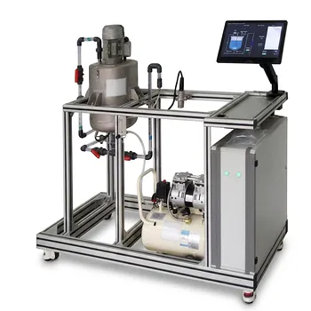
What Assumptions Apply To Tubular Reactor Axial Dispersion Models? A Lab Guide.

Here’s the straightforward truth about what those tubular reactor training units are actually built to demonstrate. When you apply the axial dispersion model to a laboratory tubular reactor, you are physically assuming three things: first, that radial concentration and temperature gradients are completely absent—the fluid is perfectly mixed in a cross‑section; second, that the fluid’s spatial velocity remains perfectly constant along the entire tube length; and third, that any spreading of mass or heat in the axial direction behaves exactly like diffusion, following Fick’s law (mass) and Fourier’s law (heat), just with effective “dispersion coefficients” that lump together all real mixing effects.

A tubular reactor training unit is not a mere plug‑flow device—it’s a physical playground where students confront how a handful of bold assumptions turn messy reality into a solvable model, directly linking fluid dynamics to the all‑important Danckwerts boundary conditions.

Why Those Three Assumptions Are the Whole Game

The axial dispersion model isn’t just a formula—it’s a deliberate simplification that lets engineers capture non‑ideal flow without drowning in computational complexity. The three assumptions aren’t accidents; they are what make the model teachable and physically interpretable in a benchtop setup.

Assumption 1: A Perfectly Uniform Cross‑Section (No Radial Gradients)

You are assuming the pipe has no “thin spots” of concentration or temperature. Every molecule at a given axial position sees the same conditions.

In a real tube, laminar or turbulent flow creates radial velocity profiles, which naturally cause radial gradients. The axial dispersion model ignores these entirely by treating the reactor as a one‑dimensional system. This is a deliberate trade‑off: it eliminates the need for a full 3D simulation, allowing students to focus on axial mixing effects while still seeing their impact on conversion.

Assumption 2: Constant Axial Velocity (No Acceleration or Deceleration)

You are assuming the fluid never speeds up or slows down. Density changes from reaction or heating, entrance effects, and boundary layer growth are all set aside.

In a training reactor, students often run isothermal liquid‑phase reactions with negligible volume change. That’s precisely the controlled condition where this assumption feels nearly true—the lab rig is built to make the model’s simplifications physically visible. When students later encounter a gas‑phase reaction with molar expansion, the mismatch between assumption and data becomes a powerful teaching moment.

Assumption 3: Axial Dispersion Follows Fick’s and Fourier’s Laws Exactly

You are assuming that mass and heat spread axially just like simple diffusion. The real‑world chaos—turbulent eddies, Taylor dispersion, molecular diffusion—gets stuffed into a single effective dispersion coefficient (Dₐ for mass, kₐ for heat).

This is the heart of the model’s practical power. Students learn that you can still use the exact same mathematical form as Fick’s law, even when the underlying physics are wildly different. The coefficient becomes a lumped “catch‑all” that an engineer can measure from a residence time distribution (RTD) experiment, no CFD required.

The Hidden Bridge: How the Assumptions Activate the Boundary Conditions

The physical assumptions aren’t just a list to memorize—they are what make the Danckwerts boundary conditions both necessary and mathematically well‑defined. Without them, the inlet and outlet conditions wouldn’t close the problem.

When you assume no radial gradients and a constant velocity, the entire reactor collapses to a single axial coordinate. At the inlet, mass jumping from an upstream plug‑flow zone into a dispersed‑flow zone must satisfy a flux continuity equation—that’s the famous Danckwerts condition. The constant‑velocity assumption ensures that the convective flux term is unambiguous, while the Fick‑like dispersion assumption gives you the diffusive flux term in a form students can integrate by hand.

From Abstract to Tangible: What the Lab Rig Physically Enforces

In a training unit, you can literally see the implications:

A long, narrow tube minimizes radial gradients naturally, making Assumption 1 a near‑reality.
A constant‑speed pump and a liquid with constant density enforce Assumption 2 at the hardware level.
A tracer injection followed by a conductivity measurement gives you an RTD curve, which, when fitted to the dispersion model, yields the effective dispersion coefficient—and Assumption 3 becomes a number, not a theory.

That sequence, from physical constraints to model parameters, is exactly the learning arc the training unit is designed to illustrate.

Understanding the Trade‑offs

Every one of those assumptions is, in a strict sense, false outside the carefully controlled lab conditions. Acknowledging that is central to building engineering judgement.

Neglecting radial gradients means the model can’t predict hot spots or wall effects. In an exothermic reaction, real radial temperature profiles can cause runaway—the model is blind to that danger.
Assuming constant velocity breaks down as soon as density changes significantly. For gas‑phase reactions with molar change, the model will systematically over‑ or under‑predict conversion.
Using an effective dispersion coefficient hides the true multiscale physics. That single number is flow‑rate‑dependent and geometry‑dependent—extrapolating it to a larger reactor without understanding its origin is a classic scaling‑up mistake.

These are not flaws in the training experience—they are the lesson. Students who wrestle with the mismatch between model prediction and experimental data leave the lab understanding where the real‑world limits lie.

Making the Most of a Tubular Reactor Training Unit

How you design the lab session determines whether students see these assumptions as brittle simplifications or as powerful, deliberate tools.

If your primary focus is building fundamental model literacy: Run multiple tracer experiments at different flow rates. Show how the effective dispersion coefficient changes, and discuss why the Fick‑like assumption still yields a usable RTD fit—even when the physics aren’t actually diffusive.
If your primary focus is connecting theory to industrial boundary conditions: Derive the Danckwerts inlet condition step‑by‑step on a whiteboard, then let students watch the reactor’s inlet flow pattern (via dye or a simple pH‑indicator tracer). Emphasize how the flux continuity only makes sense under Assumptions 1 and 2.
If your primary focus is teaching the limits of simplification: Deliberately break an assumption: run a reaction with a sudden density change, or introduce a high‑viscosity fluid that develops noticeable radial velocity profiles. Then ask students to explain why the axial dispersion model fails—and what an engineer would need to do instead.

A training reactor is never just about plug flow; it’s a carefully staged argument that the most teachable models are built on a handful of brave, falsifiable physical assumptions—and recognizing them is what separates a button‑pusher from a problem‑solver.

Summary Table:

Key Assumption	Physical Meaning	Practical Limitation
No Radial Gradients	Uniform concentration and temperature across the pipe cross-section.	Cannot predict radial hot spots or wall effects.
Constant Axial Velocity	Fluid velocity remains constant; no acceleration or density changes.	Fails under significant density changes (e.g., gas-phase reactions).
Fickian/Fourier Dispersion	Axial mixing and heat spreading behave like simple diffusion.	Lumps complex physics into a single, flow-dependent coefficient.

Bridge Engineering Theory and Practice with LABPARK

Looking to equip your laboratory with training systems that clearly illustrate complex thermodynamics and fluid dynamics? LABPARK provides premium Educational and Vocational Unit Operations Pilot Plants in chemical engineering, bioprocess & biotech, and environmental & water treatment for universities, research institutes, and enterprises.

Our robust pilot plants help students visualize physical assumptions—like dispersion and heat transfer—in real-world, hands-on setups.

Contact LABPARK today to discuss your laboratory equipment needs and request a custom quote!