What Correlations Calculate Mass Transfer In Gas Absorption Pilot Plants? Key Parameters Explained

Selecting the right mass transfer model is the first step in translating pilot plant data into reliable design principles. In educational gas absorption packed columns, the gas-film mass transfer coefficient ($k_G$) is typically estimated using a power-law correlation based on dimensionless groups: $Sh_G = \alpha (Re_G)^\beta (Sc_G)^\gamma$, where $\alpha$, $\beta$, and $\gamma$ are packing-specific constants. The liquid-film coefficient ($k_L$) often follows a specific form such as $Sh_L = 0.00595 (Re_L)^{0.67} (Sc_L)^{0.33} (Ga)^{0.33}$. To apply either correlation, you must measure superficial phase velocities, temperature, pressure, fluid viscosities, densities, diffusivities, and the geometric characteristics of the packing.

These empirical correlations act as a bridge between measurable bulk flow conditions and the local interfacial transport you cannot probe directly. They work only as well as the data you feed them, and their accuracy hinges on using packing-specific constants within their validated operating envelope.

Why Dimensionless Groups Dominate Mass Transfer Modeling

The Fundamental Driving Forces

Mass transfer coefficients are not constants—they shift with fluid dynamics and solute properties. Using dimensionless numbers collapses a complex multivariable problem into a manageable form. The Sherwood number ($Sh$) is the dimensionless mass transfer coefficient, while the Reynolds number ($Re$) accounts for flow regime and turbulence. The Schmidt number ($Sc$) links momentum and mass diffusivity, and the Galileo number ($Ga$) adds gravitational and liquid-film effects for gravity-driven flow over packing.

A Practical Bridge Between Theory and Experiment

These correlations are derived from decades of experiments with specific packings. They let students calculate $k_G$ and $k_L$ without direct interfacial imaging. By measuring only bulk velocities, fluid properties, and packing size, the correlation outputs a coefficient that can be used immediately in HTU/NTU analysis or rate calculations.

The Gas-Film Correlation: $Sh_G = \alpha (Re_G)^\beta (Sc_G)^\gamma$

Generic Form and Packing-Specific Constants

The gas-phase Sherwood number is expressed as $Sh_G = \frac{k_G d_p}{D_G}$, where $d_p$ is a characteristic packing dimension and $D_G$ is gas diffusivity. The constants $\alpha$, $\beta$, and $\gamma$ are not universal—they come from published data for materials like Raschig rings, Berl saddles, or structured packings. You must pick the correlation set that matches the exact packing in your educational column.

Parameters You Must Measure

To compute $Re_G$ and $Sc_G$, you need the superficial gas velocity (gas volumetric flow rate divided by column cross-sectional area), the gas-phase viscosity and density (from temperature and pressure), and the solute diffusivity in the gas (often estimated from kinetic theory). The packing nominal size or equivalent diameter provides $d_p$.

The Liquid-Film Correlation: $Sh_L = 0.00595 (Re_L)^{0.67} (Sc_L)^{0.33} (Ga)^{0.33}$

A Semi-Empirical Classic

This specific numerical form appears frequently for random packings at moderate liquid loads. Here $Sh_L = \frac{k_L d_p}{D_L}$, $Re_L$ uses the superficial liquid velocity and liquid properties, $Sc_L = \frac{\mu_L}{\rho_L D_L}$, and $Ga = \frac{d_p^3 g \rho_L^2}{\mu_L^2}$. The inclusion of the Galileo number accounts for liquid film drainage under gravity, a phenomenon that influences film thickness and exposure time.

How the Galileo Number Shapes Liquid-Side Resistance

Ga multiplies inside the correlation, effectively making $k_L$ depend on $d_p^{1.33}$ and fluid properties. A larger packing piece or higher density boosts Ga, increasing predicted $k_L$. This reflects the fact that on larger packing elements, liquid films often travel faster and are more disrupted, enhancing transport.

Essential Parameters You Absolutely Must Measure

Superficial Phase Velocities

Both correlations demand the superficial gas velocity and superficial liquid velocity. Measure gas and liquid volumetric flow rates with rotameters or mass flow controllers, then divide by the empty column cross-sectional area. These are your direct inputs to $Re_G$ and $Re_L$.

Fluid Physical Properties

Viscosity, density, and diffusivity for both phases must be known at the operating temperature and pressure. For common educational systems (CO₂–water–air), use literature correlations or simple lab measurements. Temperature and pressure sensors on the column are non-negotiable because properties can shift noticeably during a run.

Packing Geometry and Column Dimensions

You need the nominal packing size (e.g., 10 mm ceramic Raschig ring) and the column internal diameter. This size becomes $d_p$ in every dimensionless group. Without an accurate packing measurement, your $Sh$ values will be unreliable regardless of flow data quality.

Concentration Data to Close the Loop

Even if the correlations give $k_G$ and $k_L$, educational setups commonly validate them by measuring inlet/outlet solute concentrations (e.g., dissolved CO₂ via titration or gas chromatography). These values feed mass balances and allow back-calculation of the overall coefficient, confirming that the dimensionless approach is consistent with observed separation.

Common Pitfalls and Trade-offs

The Empirical Ceiling

Correlations like $Sh_L = 0.00595 (Re_L)^{0.67}...$ are only valid within the range of conditions used to derive them. Pushing far beyond original flow rates, liquid viscosities, or packing sizes can give physically impossible coefficients. Never extrapolate blindly.

Packing Constants Matter More Than You Think

Using generic $\alpha, \beta, \gamma$ values for the wrong packing type can introduce errors larger than 30%. If your column contains modern high-surface-area packings, the constants from 1960s-era Raschig ring data will mislead you. Always match the correlation source to the packing supplier’s data or an established reference like Onda’s correlations.

The Hidden Cost of Poor Diffusivity Estimates

Schmidt numbers rely on diffusivity. In educational labs, students often approximate gas diffusivity with simple kinetic theory formulas and liquid diffusivity with the Wilke-Chang correlation. Small errors here propagate into $Sh$, so dedicated experiments or careful property lookups are well worth the effort.

Flooding and Flow Regime Boundaries

The correlations implicitly assume pre-loading or loading conditions. Once the column enters the flooding region, the simple $Re$ exponent no longer captures the chaotic hydrodynamics. Always monitor pressure drop and liquid holdup to ensure you stay inside the usable operating envelope.

Making the Right Choice for Your Educational Setup

Different learning objectives call for different emphasis when applying these correlations. Use the following guide to focus your measurements and analysis.

If your primary focus is illustrating gas-film controlled absorption: Concentrate on accurate gas-phase velocity and diffusivity data, and verify the correlation against systems like ammonia–air–water, where liquid resistance is minor.
If your primary focus is exploring liquid-film resistance: Prioritize liquid property measurements and use the liquid-phase correlation with Galileo number. Systems such as CO₂–water are ideal because liquid-side resistance dominates.
If your primary focus is comparing packing performance: Keep the same fluid system and vary only the packing. Use the correlation constants for each packing type while rigorously measuring identical flow conditions.
If your primary focus is validating HTU and NTU design methods: Combine the dimensionless $k$-coefficients with known interfacial area correlations to predict column height, then compare with direct concentration profile data.

Each choice starts from the same dimensionless foundation. Master the measurements, respect the empirical limits, and your pilot plant will deliver industrial-grade insight.

Summary Table:

Phase	Correlation Form	Key Dimensionless Groups	Crucial Measured Parameters
Gas-Film	$Sh_G = \alpha (Re_G)^\beta (Sc_G)^\gamma$	Sherwood ($Sh_G$), Reynolds ($Re_G$), Schmidt ($Sc_G$)	Gas velocity, temperature, pressure, gas viscosity/density, solute diffusivity, packing size
Liquid-Film	$Sh_L = 0.00595 (Re_L)^{0.67} (Sc_L)^{0.33} (Ga)^{0.33}$	Sherwood ($Sh_L$), Reynolds ($Re_L$), Schmidt ($Sc_L$), Galileo ($Ga$)	Liquid velocity, temperature, liquid viscosity/density, solute diffusivity, packing size

Elevate Chemical Engineering Education with LABPARK

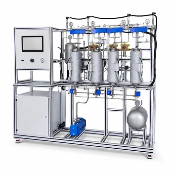
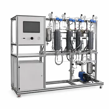
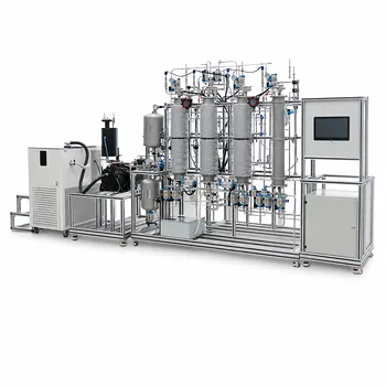
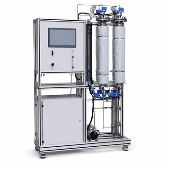
Looking to provide your students with hands-on experience in mass transfer and fluid dynamics? LABPARK provides premium Educational and Vocational Unit Operations Pilot Plants in chemical engineering, bioprocess & biotech, and environmental & water treatment for universities, research institutes, and enterprises.

Our advanced gas absorption pilot plants deliver:

High-Precision Data: Integrated sensors ensure accurate measurement of velocities, temperatures, and pressures to simplify correlation calculations.
Versatile Configurations: Easily swap packings and test different liquid/gas ratios to validate $Sh$, $Re$, and $Sc$ calculations.
Robust Curriculum Support: Turnkey solutions that bridge complex mass transfer theory with practical laboratory experience.

Bring industry-grade insight into your educational labs. Contact LABPARK today to explore our pilot plant solutions and request a custom quote!