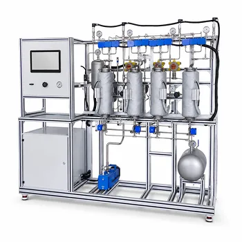
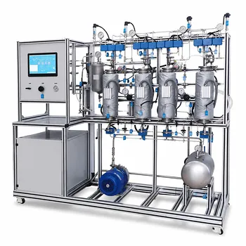
Why Account For Absorption Factor Variations? Accurate Calculations For Gas Absorption Pilot Plants.

Here’s the simple truth: a single absorption factor cannot describe reality because temperature and flow conditions change continuously from the top to the bottom of the column.
You must account for these variations when analyzing pilot plant experiments; otherwise, your calculated mass transfer performance will be inaccurate and mislead scale‑up decisions. The accepted engineering practice is to replace the single absorption factor with the geometric mean of the absorption factors at the column’s top and bottom, then apply the Kremser equation to extract the number of theoretical stages or transfer units. This bridges the gap between ideal column models and the thermal and hydrodynamic realities you observe in a pilot absorber.

Core Takeaway
In real pilot‑scale absorption, heat effects and solute transfer cause the equilibrium constant and the operating line slope to change along the column. Relying on one absorption factor distorts performance calculations. The solution is to measure top‑ and bottom‑conditions, compute the geometric mean absorption factor, and use that single representative value in the analytical Kremser equation—a method that is both standard and practical for training and research.

Why the Absorption Factor Varies in a Pilot Column

The absorption factor (A = L / mV) is the ratio of the operating line slope (L/V) to the equilibrium line slope (m). Both the numerator and the denominator can drift as gas and liquid travel through the packed height.

Temperature-Driven Changes in Equilibrium

In a pilot plant, absorption is almost never isothermal.
The molar heat of absorption or reaction releases energy, causing a measurable temperature rise along the column.
Since the equilibrium constant m (Henry’s law constant) is strongly temperature‑dependent, a hotter bottom section gives a larger m—thus a lower local A—than the cooler top tray.
If you ignore this, the average driving force you assume stays flat while the real driving force shrinks in the lower bed.

Flow Rate Variations from Solute Transfer

As solute moves from the gas into the liquid, the liquid flow rate L increases slightly downward and the gas flow rate V decreases upward.
These changes in L and V alter the internal L/V ratio.
In a pilot column treating a concentrated gas, the variation can be significant enough that a single operating line slope no longer matches the true internal profile.

The Problem with Using a Single Absorption Factor

Plugging one value of A into a standard stage‑wise calculation (e.g., Kremser) assumes a uniform equilibrium and a straight operating line.
Real temperature and flow profiles bend both lines. The resulting error can lead to:

Over‑ or under‑estimating the number of theoretical stages.
You might conclude that a pilot column has much more or less capacity than it actually delivers.
Misleading scale‑up.
A design based on a single‑A model from cool, dilute inlet conditions will fail when the industrial unit heats up and concentrates the solute.

Objective analysis of pilot plant data absolutely requires a method that respects these gradients.

How to Account for Variation: The Geometric Mean Approach

The standard, teachable fix is to treat the column not with one absorption factor but with the geometric mean of the factors at the two ends.
This gives you a single number that represents the average absorption power across the entire bed.

Calculating the Geometric Mean Absorption Factor

Collect four pieces of data from the pilot plant:

Liquid and gas flow rates (L, V) and compositions at the top to get A_t
The same flows and compositions at the bottom to get A_b

Then compute:

[ A_{\text{geometric}} = \sqrt{A_t \cdot A_b} ]

This form acknowledges that A often changes exponentially along the height, especially when the equilibrium line curves. The square root of the product is the proper mathematical average when variations follow a log‑linear path.

Applying the Analytical Kremser Equation

Once you have A_geometric, you can use the standard analytical Kremser equation for a lean‑end or rich‑end correction.
For a typical absorption problem (solute transferred from gas to liquid), the number of theoretical stages or transfer units becomes:

[ N = \frac{\ln!\left[\left(\frac{1 - 1/A}{y_{\text{in}} - m x_{\text{in}}}\right) \cdot \frac{y_{\text{out}} - m x_{\text{in}}}{y_{\text{in}} - m x_{\text{in}}} + \frac{1}{A}\right]}{\ln A} ]

(where the A used inside the equation is the geometric mean A).

Alternatively, for packed columns, you can convert to the number of overall transfer units N_OG. The key is that the same geometric mean A is inserted into the log‑mean driving force correction.

In the lab, students measure inlet/outlet temperatures and concentrations, calculate A_t and A_b, find the geometric mean, and then solve the Kremser equation for N. This lets them compare experimental stage efficiencies directly with theoretical predictions, accounting for the real temperature bulge.

Understanding the Trade‑offs

The geometric mean method is widely used and fits excellently into pilot‑plant education, but it is still an engineering approximation.

Non‑linear profiles. If the temperature profile has a sharp hump (often seen with chemical absorption), a simple top‑bottom average may under‑predict the true number of stages.
Flow measurement accuracy. Small errors in L or V at either end propagate into A_geometric. Pilot plants need properly calibrated rotameters and temperature probes.
Desorption‑driven loops. In a closed‑cycle solvent system (absorber + stripper), the lean solvent returning to the top is rarely perfectly clean, which shifts the top A. You must measure both columns to get representative flow conditions.
When a single A fails silently. If your calculated geometric mean A is far from the arithmetic mean, it signals strong curvature; in that case, a segment‑by‑segment numerical integration gives better insight, though it demands more sampling points.

Despite these caveats, for training and early‑stage scale‑up, the geometric mean method strikes an ideal balance between physical reality and computational simplicity.

Making the Right Choice for Your Pilot Plant Data Analysis

How you handle the absorption factor depends on what you need from the experiment.

If your primary focus is teaching fundamental column dynamics: Use the geometric mean A method with top‑ and bottom‑only measurements. It cleanly demonstrates why a single A is insufficient and shows students how heat effects distort stage numbers—exactly the lesson a pilot plant is meant to deliver.
If your primary focus is high‑fidelity model validation: Consider installing axial temperature sensors and taking side‑stream samples. Then, perform a stage‑by‑stage or short‑segment integration where A is recalculated at each height. This yields a more accurate N and accounts for sharp thermal gradients, though it requires more time and instrumentation.
If your primary focus is comparing solvents or operating conditions: Stick to the geometric mean approach but ensure you record inlet/outlet conditions meticulously for each run. The consistent method allows fair comparisons of stage efficiency at different L/V ratios, even if the absolute accuracy is slightly lower.

Remember: The goal isn’t to eliminate variation in the absorption factor—it’s to measure it and fold it into your analysis so that your pilot‑scale conclusions become a trustworthy bridge to the full‑scale plant.

Summary Table:

Parameter Variation	Cause in Pilot Plant	Recommended Solution
Equilibrium Constant (m)	Temperature rise from heat of absorption	Calculate the geometric mean: $A_{\text{geometric}} = \sqrt{A_t \cdot A_b}$
Flow Rates (L, V)	Solute transfer changing phase flow rates	Apply $A_{\text{geometric}}$ directly in the Kremser equation

Optimize Your Engineering Labs with LABPARK

Accurate data analysis starts with reliable equipment. LABPARK provides state-of-the-art Educational and Vocational Unit Operations Pilot Plants in chemical engineering, bioprocess & biotech, and environmental & water treatment.

Engineered for universities, research institutes, and enterprises, our pilot plants feature precise instrumentation and reliable controls to help your students and researchers master complex mass transfer concepts with ease.

Ready to upgrade your laboratory capabilities? Contact LABPARK today to explore our custom solutions!