The filtration or hydration time through a semipermeable membrane is quantified using the integrated volumetric flow equation: (t_{hydrate} = \frac{V_d h_0}{4\pi r_0^2 L_p \sigma \Delta\Pi}). In a pilot-plant setting, this formula lets you calculate the exact time required for a specific volume of permeate ((V_d)) to pass through the membrane, based on the membrane’s physical properties and the osmotic driving force. By systematically altering parameters like membrane thickness ((h_0)) or permeability ((L_p)), you can directly observe and measure the rate-limiting steps in mass transfer.
The core of the calculation captures the interplay between membrane resistance, available surface area, and the osmotic gradient. The equation reveals that hydration time is not a fixed property—it is a dynamic outcome of the chosen membrane material and the applied experimental conditions, allowing you to precisely model and predict membrane performance.
Deconstructing the Hydration Time Equation
The formula derived from the primary reference is built on a steady-state model of transmembrane flux. Understanding each component is essential for meaningful data interpretation in a pilot plant.
The Driving Force: Osmotic Pressure Difference ((\Delta\Pi))
(\Delta\Pi) represents the net osmotic pressure difference between the feed and permeate sides. It is the thermodynamic “push” that moves solvent across the membrane against a concentration gradient. In processes like reverse osmosis, a hydraulic pressure must overcome this osmotic difference, and the portion that actually drives flow is often proportional to (\Delta\Pi) in models where a reflection coefficient is used.
The Membrane’s Resistive Properties: (L_p), (\sigma), and (h_0)
The membrane permeability coefficient ((L_p)) is a measure of how easily solvent can flow through the membrane structure per unit area and pressure. It is an intrinsic property that depends on pore size, porosity, and material chemistry.
The reflection coefficient ((\sigma)) ranges from 0 to 1 and indicates the membrane’s ability to reject solute. A value of 1 means the solute is perfectly reflected, making the full osmotic pressure effective. A lower value reduces the effective driving force, as solute leaks through.
The membrane thickness ((h_0)) appears in the numerator because resistance to flow increases linearly with thickness. A thicker membrane directly increases the hydration time, assuming other factors remain constant.
The Geometric Factor: Surface Area ((4\pi r_0^2))
The term (4\pi r_0^2) represents the surface area of the membrane if modeled as a sphere of initial radius (r_0). In a pilot plant, this factor highlights that scaling up or down requires accounting for the available area. A larger area decreases hydration time for a given volume because more parallel flow paths exist. The spherical assumption might be adapted in practice to flat-sheet or cylindrical geometries, but the principle remains: flow rate is proportional to area.
The Volume Target: (V_d)
(V_d) is the volume of permeating fluid you aim to collect. It sets the endpoint of your experiment. The equation shows that hydration time scales linearly with this target volume—doubling the target volume doubles the time needed, provided other conditions stay constant.
Applying the Calculation in a Pilot Plant Setting
Your pilot plant’s value lies not just in running the experiment, but in using this equation to design it and dissect the results.
Designing a Controlled Experiment
Begin by fixing all known parameters that you can measure or calibrate. Steady-state conditions are assumed, so your system must reach equilibrium before (t_{hydrate}) is meaningful. If you vary (L_p) by testing different membrane types or (\Delta\Pi) by changing feed concentration, the equation predicts the new hydration time.
Step-by-Step Calculation in Practice
- Characterize the membrane: Obtain or measure (L_p) and (\sigma) for your specific membrane and solute pair. The pilot plant may help you determine these values through separate experiments.
- Determine the geometry: Measure the effective membrane surface area. If using a tubular or flat-sheet module, convert the area equivalent to the spherical model or derive a new geometric factor.
- Calculate osmotic pressure: Use feed and permeate concentration data to compute (\Delta\Pi) (e.g., using the van’t Hoff equation for dilute solutions).
- Plug in the target volume: Choose (V_d) carefully—too large and the assumption of constant (\Delta\Pi) may break down; too small and measurement errors dominate.
- Solve for (t_{hydrate}). Compare this theoretical value with your observed time to assess model accuracy or membrane fouling.
Linking the Calculation to Broader Membrane Processes
The supplementary references illustrate that this type of calculation is most directly applicable to pressure-driven processes like nanofiltration and reverse osmosis, where osmotic pressure plays a central role. For microfiltration or ultrafiltration where osmotic effects are negligible, the driving force is primarily the applied hydraulic pressure, and a simplified Darcy-type equation would replace (\sigma \Delta\Pi). Understanding this context helps you select the right model for your specific module within the pilot plant.
Understanding the Trade-offs and Limitations
Every model involves assumptions. Vigilance about these will prevent misapplying the equation.
Assumption of Constant Parameters
The equation assumes (L_p), (\sigma), and (\Delta\Pi) remain constant during the experiment. In reality, concentration polarization can increase the effective osmotic pressure at the membrane surface, and membrane fouling can reduce (L_p) over time. This causes the actual hydration time to drift from the theoretical prediction, so your pilot plant must include proper flow management and cleaning protocols.
The Spherical Geometry Assumption
The form (4\pi r_0^2) is specific to a spherical core. Most pilot plant modules use spiral-wound, hollow-fiber, or flat-sheet configurations. Applying this equation directly will introduce error unless you properly translate the geometry into an equivalent surface area. The underlying physics (flow proportional to area) holds, but the geometric factor must be recalibrated to your module’s design.
Pore Size and Separation Regime Limits
As the supplementary references highlight, the spectrum from microfiltration to reverse osmosis changes the dominant transport mechanism. The hydration time equation is built on a solution-diffusion or pore-flow model with an explicit osmotic term. It is not suitable for purely pressure-driven microfiltration of large particles, where sieving dominates and (\sigma \approx 0). Forcing its use there would make (t_{hydrate}) inversely proportional to a vanishingly small term, yielding nonsensical values.
Measurement Uncertainty in (V_d) and (r_0)
Small errors in measuring the initial radius or the permeate volume propagate exponentially or linearly. In a teaching pilot plant, this is an opportunity to discuss precision, calibration, and error analysis. Encourage repeated trials and careful documentation to build statistical confidence in your reported hydration time.
Making the Right Choice for Your Pilot Plant Study
Use this equation and your pilot plant as a diagnostic tool, not just a recipe. Adapt your approach based on what you need to learn about the membrane.
- If your primary focus is characterizing a new membrane: Perform multiple hydration time experiments at different (\Delta\Pi) values to back-calculate (L_p) and (\sigma). Use the results to benchmark against other materials.
- If your primary focus is predicting large-scale performance: Use the pilot plant to validate the equation under realistic feed conditions, then scale the surface area term accordingly. Watch for fouling trends that alter the effective (L_p) over time.
- If your primary focus is understanding mass transfer fundamentals: Vary (h_0) or solute type systematically and plot the resulting hydration times. Connect the observed trends back to the governing equation to solidify theoretical concepts.
- If your primary focus is operator training or education: Use the clear, direct calculation to let users see the impact of each variable in isolation, reinforcing the relationship between membrane properties and separation efficiency.
With this equation as your foundation, your pilot plant transforms from a mere assembly of pumps and tubes into a precise instrument for membrane science.
Summary Table:
| Variable | Symbol | Description | Impact on Hydration Time |
|---|---|---|---|
| Target Volume | $V_d$ | Volume of permeate to collect | Directly proportional (increases time) |
| Membrane Thickness | $h_0$ | Thickness of the membrane | Directly proportional (increases time) |
| Membrane Surface Area | $4\pi r_0^2$ | Active area modeled on initial radius $r_0$ | Inversely proportional (decreases time) |
| Permeability Coefficient | $L_p$ | Ease of solvent flow through membrane | Inversely proportional (decreases time) |
| Reflection Coefficient | $\sigma$ | Membrane's solute rejection capability | Inversely proportional (decreases time) |
| Osmotic Pressure Diff. | $\Delta\Pi$ | Net thermodynamic driving force | Inversely proportional (decreases time) |
Bring Theory to Life with LABPARK Pilot Plants
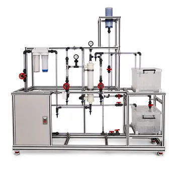
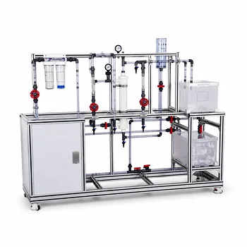
Bridge the gap between theoretical membrane transport equations and hands-on laboratory experience. LABPARK provides state-of-the-art Educational and Vocational Unit Operations Pilot Plants in:
- Chemical Engineering (including advanced membrane separation systems)
- Bioprocess & Biotech
- Environmental & Water Treatment
Designed specifically for universities, research institutes, and enterprises, our scalable systems offer real-world training on filtration calculations, mass transfer, and process design.
Contact LABPARK today to discover how our pilot plants can elevate your research and teaching capabilities!
Related Products
- Multi-Functional Membrane Separation Educational Pilot Plant for Unit Operations Lab
- Photocatalytic Membrane Separation and Degradation Unit Operations Pilot Plant
- Ultrafiltration Membrane Separation Educational Pilot Plant
- Multifunctional Membrane Separation Educational Pilot Plant with Ultrafiltration, Nanofiltration, Reverse Osmosis
- Hollow Fiber Ultrafiltration Membrane Separation Educational Pilot Plant
People Also Ask
- What are the key differences in membrane configurations? Choose the Right Unit Operations Pilot Plant
- How Do Pervaporation, Vapor, and Gas Permeation Differ in Pilot Plants? Key Comparison
- What are the advantages of membrane separation pilot plants? Energy-saving process intensification.
- Pervaporation vs. Vapor Permeation: Handling Suspended Solids in Membrane Pilot Plants
- How do PEI, PVDF, and PSU membranes compare in pilot plants? Find the best fit.