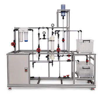
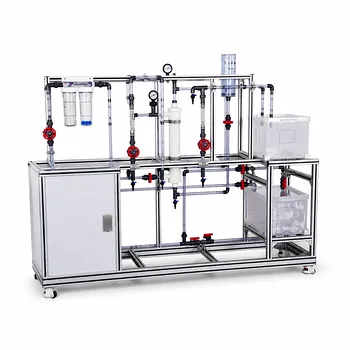
How To Determine Specific Cake (R) & Filter Medium (Rm) Resistance Using Filtration Pilot Plant Data

By transforming raw pilot plant data into a simple linear plot, you can directly extract the two fundamental resistances that govern filtration performance. In a constant-pressure filtration run on a pilot plant, you determine specific cake resistance (r) from the slope of a $\frac{d\theta}{dV}$ versus $V$ plot, and filter medium resistance ($R_m$) from the intercept. This method relies on the linearized filtration equation and real-time measurements of filtrate volume and time under a fixed pressure drop.

The core strategy for determining r and $R_m$ is to operate the pilot plant at constant pressure, record cumulative filtrate volume ($V$) as a function of time ($\theta$), and then use numerical differentiation to construct a plot of $\frac{d\theta}{dV}$ against $V$. The straight-line relationship that emerges directly yields both resistance values through its slope and intercept.

The Foundation: The Constant-Pressure Filtration Equation

The Governing Equation in a Pilot Plant

The behavior of any pressure-driven filtration is captured by the differential equation that balances the applied pressure drop with the sum of cake and medium resistances. For a constant-pressure operation, this equation is linearized as:

$$\frac{d\theta}{dV} = \frac{\mu r v}{A^2 \Delta p} V + \frac{\mu R_m}{A \Delta p}$$

Here, $\mu$ is the filtrate viscosity, $v$ is the volume of cake deposited per unit volume of filtrate, $A$ is the filter area, and $\Delta p$ is the constant pressure drop. The equation shows that the inverse filtration rate ($\frac{d\theta}{dV}$) increases linearly with the cumulative filtrate volume ($V$) because the growing cake adds resistance.

How Pilot Plant Data is Collected

A modern unit operations pilot plant logs time and volume data automatically using sensors and data acquisition systems. Students and researchers simply set a constant back-pressure regulator or control valve to maintain $\Delta p$, then start the run. The system records the time required to collect successive, equal volumes of filtrate. These raw $\theta$–$V$ pairs are the only experimental input you need to determine both resistances.

Why a Constant Pressure Drop is Essential

The method assumes a strictly constant $\Delta p$ throughout the run. Any fluctuation in pressure makes the linear relationship invalid, because the slope term then contains a time-varying $\Delta p$. A well-designed pilot plant uses a pressurized feed tank and a precision regulator to lock in the target pressure, ensuring the data fits the model.

The Graphical Method: From Experimental Data to Resistances

Step 1: Calculate the Instantaneous Filtration Rate

You first need values of $\frac{d\theta}{dV}$ at several points. In practice, this is done by numerical differentiation of your $\theta$–$V$ data. For each measured volume increment $\Delta V$, calculate the corresponding time increment $\Delta \theta$, and then compute $\frac{\Delta \theta}{\Delta V}$ as an approximation of the derivative. Use the cumulative volume $V$ at the midpoint of the interval for the plot.

Step 2: Plot dθ/dV vs. Cumulative Volume (V)

Place the calculated $\frac{d\theta}{dV}$ values on the y-axis and the associated cumulative filtrate volumes on the x-axis. If the cake is relatively incompressible and the data is clean, the points will fall on a straight line, confirming the validity of the constant-pressure model. Deviations from linearity often point to cake compressibility or early-time disturbances.

Step 3: Extract Slope and Intercept

Perform a linear regression on the plotted points. The slope of this line is $K = \frac{\mu r v}{A^2 \Delta p}$, and the y-intercept is $C = \frac{\mu R_m}{A \Delta p}$. These two numbers contain all the information needed to calculate the resistances.

Step 4: Solve for r and Rm

Rearrange the expressions to isolate the unknowns. Specific cake resistance $r$ is obtained as:

$$r = \frac{K \cdot A^2 \Delta p}{\mu v}$$

Filter medium resistance $R_m$ follows from the intercept:

$$R_m = \frac{C \cdot A \Delta p}{\mu}$$

You must know the slurry property $v$ (often determined by a simple material balance on solids concentration in feed and cake) and the fluid viscosity $\mu$ at the operating temperature. The pilot plant data now yields two intrinsic, scalable parameters that characterize the filtration system.

Interpreting the Results: What r and Rm Tell You

Specific Cake Resistance (r) and Filtration Speed

The value of $r$ is not just a number—it categorizes the filterability of your slurry. In conventional equipment, a specific cake resistance in the range of $10^7$–$10^8$ m/kg indicates fast filtering, while values above $10^{10}$ m/kg signal very slow filtering. This parameter is an intrinsic property of the solid particles, reflecting their size, shape, and how they pack. A high $r$ warns that you may need a larger filter area, a higher pressure (if the cake is incompressible), or a pre-treatment step like adding a filter aid.

Filter Medium Resistance ($R_m$) and Its Diminishing Role

$R_m$ dominates only at the very start of filtration, when no cake has formed. As soon as a thin layer of solids accumulates, the cake resistance $\frac{\mu r v V}{A^2 \Delta p}$ overshadows the medium term. In a typical pilot run, the medium resistance becomes negligible after the first few seconds, which is why the y-intercept often appears small. Nevertheless, knowing $R_m$ is critical for selecting the right cloth or membrane and for predicting initial flow rates during plant start-up.

Understanding the Trade-offs and Pitfalls

The Compressibility Factor

The straight-line method works perfectly for incompressible cakes where $r$ is independent of pressure. For compressible materials (e.g., soft metal oxides), the specific cake resistance increases with $\Delta p$. A single constant-pressure run gives an apparent $r$ valid only at that pressure. To fully characterize such a material, you must perform multiple runs at different $\Delta p$ values, then plot $\log(\text{slope})$ versus $\log(\Delta p)$ to find the compressibility index $s$. Applying a one-point result without this check can lead to serious scale-up errors.

Data Quality and Numerical Differentiation

The calculation of $\frac{\Delta \theta}{\Delta V}$ amplifies noise in the raw time-volume data. Using very small volume increments leads to erratic derivative values, while overly large increments mask the cake buildup trend. In a pilot plant, it is often better to collect data at moderate, equal volume intervals and to use smoothing or a moving-window regression to get a clean slope. Modern data acquisition software frequently handles this differentiation internally, but manual checks remain essential.

Pilot Plant Scale vs. Industrial Reality

A pilot plant run assumes ideal plug flow and uniform cake formation. In full-scale equipment, uneven slurry distribution, cloth blinding, or cake cracking can make the $R_m$ and $r$ values drift during a batch. Pilot-derived resistances are best used as comparative benchmarks or initial design estimates. They must be validated with industrial trials for critical processes.

Making the Right Choice for Your Pilot Plant Study

The data you collect and the analysis you perform should align with your specific objective.

If your primary focus is teaching unit operations principles: Use the graphical method to demonstrate the linearized model. Have students numerically differentiate the data themselves to build an instinct for the relationship between cake growth and flux decline.
If your primary focus is characterizing a new, rigid filter cake for equipment sizing: A single careful constant-pressure run gives you a reliable $r$ for that pressure. Combine it with a known $R_m$ to calculate required filter area and batch cycle times.
If your primary focus is optimizing a compressible, slow-filtering slurry: Run the experiment at three or more pressure levels. Determine both $r$ at each pressure and the compressibility index. Use these insights to decide whether a filter aid pre-coat or a lower operating pressure is the cheaper route to higher throughput.
If your primary focus is selecting or troubleshooting the filter medium: Pay close attention to the y-intercept ($R_m$) from multiple runs. A sudden increase in $R_m$ over time can indicate medium blinding, requiring a wash step or medium replacement.

The very act of running the pilot plant transforms an abstract theory into two concrete numbers that govern your downstream decisions—so treat each data point as a direct window into your process.

Summary Table:

Parameter	Symbol	Source from Linear Plot	Formula	Physical Significance
Specific Cake Resistance	$r$	Derived from Slope ($K$)	$r = \frac{K \cdot A^2 \Delta p}{\mu v}$	Reflects slurry filterability and particle packing behavior.
Filter Medium Resistance	$R_m$	Derived from Intercept ($C$)	$R_m = \frac{C \cdot A \Delta p}{\mu}$	Dominates during initial filtration; indicates medium/cloth health.

Bring Practical Filtration Dynamics to Your Facility

Looking to equip your students or researchers with industry-ready process engineering skills? LABPARK provides premium Educational and Vocational Unit Operations Pilot Plants in chemical engineering, bioprocess & biotech, and environmental & water treatment. Our highly precise pilot systems enable universities, research institutes, and enterprises to accurately model filtration resistance, perform scale-up studies, and bridge the gap between theory and industrial practice.

Ready to elevate your laboratory capabilities? Contact LABPARK today to find the perfect pilot plant solution for your needs!