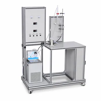
How Does A Static Vle Apparatus Determine Phase Behavior Without Vapor Sampling? Thermodynamic Modeling Explained.

The static method determines phase behavior by building a precisely known liquid composition and measuring the total pressure—then using thermodynamic consistency to calculate the vapor composition instead of extracting it.

The core insight: a low‑pressure static VLE apparatus avoids disturbing vapor–liquid equilibrium by never opening the cell to sample the vapor. It constructs an accurate P–x map from a series of liquid injections and measured pressures, and then back‑calculates the unknown vapor‑phase composition through rigorous model‑based consistency relations—a trade that sacrifices direct composition measurement for unmatched equilibrium integrity.

How the Static Apparatus Constructs a P–x Data Set

Starting from a Single Pure Component

The cell is evacuated and charged with a known quantity of one pure liquid.
It is brought to the target temperature, and its pure‑component vapor pressure is recorded.
This step not only gives the first data point but also verifies the temperature control and pressure transducer.

Injecting the Second Component with Precision

A calibrated piston‑injector delivers an exact volume of the second liquid component.
Because the density of the injectate is known, the added mass—and thus the number of moles of the second species—is known to high accuracy.
After each injection, the total moles of each component inside the cell are calculable, so the liquid‑phase mole fraction (x) is precisely determined without ever sampling the liquid.

Measuring the New Equilibrium Pressure

Once injected, the mixture is stirred and allowed to reach thermal and phase equilibrium.
The total pressure is read by a sensitive transducer.
Repeating the injection‑and‑measure step systematically builds a set of (P) versus (x) data points—all inside a hermetically sealed, static cell.

How the Vapor‑Phase Composition Is Calculated Without Sampling

The Thermodynamic Key: Model‑Based Consistency

The static cell does not measure (y) directly. Instead, the (P)–(x) data are used to fit an activity coefficient model (e.g., Margules, Wilson, NRTL) via the Gibbs‑Duhem relation.
The core idea: at equilibrium, the total pressure and the liquid‑phase activity coefficients are coupled mathematically.
Once the model parameters are optimized to match the measured pressures, the model calculates the vapor‑phase mole fractions (y) that would produce those pressures at the known (x).

A Concrete Calculation Pathway

The most common approach is Barker’s method:

Assume a form for the excess Gibbs energy with adjustable parameters.
At each (x), use the model to compute the activity coefficients and the bubble‑point pressure (the pressure at which a liquid of that composition begins to boil).
Minimize the difference between the calculated bubble pressures and the experimental (P) values.
When the fit converges, the vapor composition is a direct output of the model at each data point—no physical sample required.

Why This Preserves Equilibrium Fidelity

Physical vapor extraction removes mass, momentarily unbalancing the system and altering the composition in the cell.
For azeotropic or close‑boiling mixtures, even a tiny disturbance can shift the measured composition noticeably.
The static method keeps the cell sealed, so the measured pressure truly reflects the equilibrium state of the original charge, yielding clean, reliable (P)–(x) data that are ideal for model development.

What Makes This Method Reliable (and Where Caution Is Needed)

Trusting the Numbers: Consistency Checks

The calculated (y) values are not accepted blindly. Researchers apply thermodynamic consistency tests—most famously the area test—to verify that the fitted model and the experimental (P)–(x) data obey the Gibbs‑Duhem relation over the whole composition range.
If the test passes, the (y) values can be considered as consistent as if they had been directly measured.

Common Sources of Error

Model selection bias: If the chosen activity coefficient model cannot represent the real mixture’s non‑ideality, the inferred (y) will be systematically wrong—no matter how precisely the pressure is measured.
Injection calibration: A miscalibrated piston‑injector propagates an error into (x), which then distorts both the model fit and the resulting (y).
Incomplete degassing: Any dissolved gas in the liquids adds to the total pressure, mimicking a vapor composition effect and corrupting the data.

Understanding the Trade‑offs of the Indirect Approach

The Strengths You Gain

Unmatched equilibrium integrity: Absolutely zero mass transfer during measurement, critical for mixtures with exotic phase behavior.
Simpler experimental setup: No need for vapor circulation, online GC, or complex sampling loops—just a precise pressure gauge and a good injection system.
High data density: You can collect dozens of points across the composition range quickly after equilibrium is reached, giving a rich (P)–(x) curve for model fitting.

The Weaknesses You Accept

Model dependency: The (y) values are only as good as the thermodynamic framework you use. They are model‑generated, not raw observations.
Slower per point: Each injection requires a waiting period for phase equilibrium, which can be minutes to hours, especially in viscous mixtures.
Primarily low‑pressure domain: The method assumes the vapor can be treated as ideal (or uses a simple virial equation). At higher pressures, vapor‑phase non‑ideality requires more complex equations of state, complicating the consistency calculation—though the same principle still holds.
No direct (y) validation: You cannot independently confirm the vapor composition without additional experiments like headspace analysis—you are putting your trust in the model’s ability to extrapolate from (P)–(x) data.

How to Apply This Knowledge in Your Own Work

The static no‑sampling method is a powerful tool, but its fitness depends on your specific goals. Here is how to align your choice with your needs:

If your primary focus is obtaining the most trustworthy phase‑equilibrium pressures: This method is ideal. It eliminates sampling artifacts and gives you a clean pressure baseline, which is often the most critical piece for designing distillation and absorption columns.
If you absolutely require experimentally measured (y) data and cannot rely on a model: You will need a different technique, such as a dynamic recirculating still with online analysis. Use the static method instead as a complementary check on the (P)–(x) data, then compare the model‑predicted (y) against directly sampled values.
If you are working with azeotropic or extracting maximum information from limited data: The static method shines. By applying advanced activity‑coefficient models and consistency tests, you can often extract a complete, consistent VLE picture from pressure data alone, greatly reducing experimental complexity.
If you plan to work at elevated pressures or need industrial‑scale accuracy: Start with a low‑pressure static study to build a baseline model, but then validate at operating conditions using a method that does sample both phases—because vapor non‑idealities grow and the model‑only approach becomes less certain.

Ultimately, the low‑pressure static VLE apparatus transforms a precision pressure gauge and a set of calibrated injectors into a full phase‑behavior mapping tool—proving that, when physics and rigorous thermodynamics guide the measurement, what you don’t sample can be just as valuable as what you do.

Summary Table:

Parameter	Static VLE Method Details
Primary Measurements	Temperature ($T$), Pressure ($P$), and Liquid Composition ($x$)
Vapor Composition ($y$)	Calculated indirectly using activity coefficient models (Barker's method)
Main Advantage	No equilibrium disturbance (no mass removed during sampling)
Key Constraints	Highly dependent on model accuracy; sensitive to degassing errors

Optimize Your Chemical Engineering & Thermodynamics Labs with LABPARK

Are you looking to enhance hands-on learning and research accuracy? LABPARK provides premium Educational and Vocational Unit Operations Pilot Plants in chemical engineering, bioprocess & biotech, and environmental & water treatment. Specifically tailored for universities, research institutes, and enterprises, our pilot plants deliver robust performance, reliable data, and realistic industrial process replication.

Ready to upgrade your laboratory setup? Contact our specialist team today to find the perfect pilot plant solution for your institution!