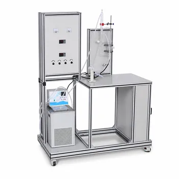
Variable time constants and static gains appear when the tank’s flow resistance changes with liquid level. In a liquid-level pilot plant with turbulent drainage, the outlet flow commonly follows (F_o=\beta\sqrt{h}), so the local process gain and time constant depend on the operating height. For control training, the usual solution is to retain the nonlinear mass-balance model for simulation while using local linear models, numerical integration, or adaptive parameter updates for controller design and analysis.

Core takeaway: A liquid-level tank with square-root outflow does not have one fixed (\tau_p) and (K_p). They must be interpreted as operating-point-dependent quantities, and training systems should show students how local approximations change as the level moves.

Why Liquid-Level Dynamics Are Nonlinear

The governing material balance

For a constant-area tank, the dynamic balance is

[ A\frac{dh}{dt}=F_i-F_o ]

where (A) is tank cross-sectional area, (h) is liquid level, (F_i) is inlet flow, and (F_o) is outlet flow.

If the outlet relationship is nonlinear,

[ F_o=\beta\sqrt{h} ]

the balance becomes

[ A\frac{dh}{dt}=F_i-\beta\sqrt{h} ]

The square-root term prevents the system from being represented exactly by one fixed first-order transfer function over all operating conditions.

Why the outlet resistance changes

The local slope of the outlet-flow relationship is

[ \frac{dF_o}{dh}=\frac{\beta}{2\sqrt{h}} ]

As the level increases, this slope decreases. In physical terms, a further increase in level produces a progressively smaller increase in outlet flow than it would at a low level.

That changing slope is the source of the variable dynamic parameters.

How the Static Gain Changes

Steady-state relationship

At steady state,

[ F_{i,s}=F_{o,s}=\beta\sqrt{h_s} ]

Therefore,

[ h_s=\left(\frac{F_{i,s}}{\beta}\right)^2 ]

The steady-state level is not proportional to inlet flow. It varies with the square of the flow, which means the process sensitivity changes with the operating point.

Local static gain

Linearizing around a steady-state level (h_s) gives

[ F_o \approx \beta\sqrt{h_s} +\frac{\beta}{2\sqrt{h_s}}(h-h_s) ]

Using deviation variables (h'=h-h_s) and (F_i'=F_i-F_{i,s}), the local model becomes

[ A\frac{dh'}{dt} +\frac{\beta}{2\sqrt{h_s}}h' =F_i' ]

The local static gain from inlet-flow deviation to level deviation is therefore

[ K_p=\frac{2\sqrt{h_s}}{\beta} ]

Thus, (K_p) increases as the operating level increases. A given change in inlet flow produces a larger ultimate level change at a higher operating level.

How the Time Constant Changes

Local first-order form

The linearized equation can be written as

[ \tau_p\frac{dh'}{dt}+h'=K_pF_i' ]

with

[ \tau_p=\frac{2A\sqrt{h_s}}{\beta} ]

Equivalently,

[ \tau_p=A R_s ]

where the local flow resistance is

[ R_s=\left(\frac{dF_o}{dh}\right)^{-1} =\frac{2\sqrt{h_s}}{\beta} ]

Physical interpretation

Because both (K_p) and (\tau_p) are proportional to (\sqrt{h_s}), the tank becomes locally slower and more sensitive as the level rises.

At a low level, the outlet-flow slope is larger, the effective resistance is lower, and the level responds more quickly. At a high level, the effective resistance is higher, so the same tank has a longer local response time.

What students should observe

For a step change near one operating point, the response may look like a conventional first-order process. The response reaches approximately 63.2% of its final value after one local time constant and approaches its final value after several time constants.

However, after a large disturbance, the changing level alters (K_p) and (\tau_p) during the response. The resulting trajectory will not follow one fixed exponential curve exactly.

Modeling Strategies for Process-Control Training

Strategy 1: Simulate the Full Nonlinear Model

Direct numerical solution

The most physically faithful model retains the original balance:

[ A\frac{dh}{dt}=F_i-\beta\sqrt{h} ]

A numerical ODE solver can calculate the level continuously as the inlet flow changes. This approach captures the changing outlet slope and does not require the process to remain close to one nominal level.

It is particularly useful for demonstrating large disturbances, startup behavior, saturation, and operation across a wide level range.

Why this approach is effective in training

A nonlinear simulation allows students to compare the actual process trajectory with a fixed first-order prediction. The difference makes the meaning of operating-point dependence visible rather than purely theoretical.

The simulator can also calculate the instantaneous or local values

[ K_p(h)=\frac{2\sqrt{h}}{\beta} ]

and

[ \tau_p(h)=\frac{2A\sqrt{h}}{\beta} ]

as the level changes.

Strategy 2: Linearize Around a Nominal Operating Point

Taylor-series approximation

For small deviations around (h_s),

[ \sqrt{h}\approx\sqrt{h_s} +\frac{1}{2\sqrt{h_s}}(h-h_s) ]

This produces the local first-order model with fixed values of (K_p) and (\tau_p) calculated at that operating point.

This is usually sufficient for controller tuning and introductory transfer-function analysis when disturbances remain small.

Use of deviation variables

Deviation variables remove the steady-state terms and focus the model on changes from the nominal condition:

[ h'=h-h_s,\qquad F_i'=F_i-F_{i,s} ]

The resulting model is easier to convert into a transfer function, state-space equation, or PID tuning form.

For the level process,

[ \frac{H'(s)}{F_i'(s)}

\frac{K_p}{\tau_p s+1} ]

This representation is convenient for teaching the relationship between physical tank properties and control-loop behavior.

Strategy 3: Use Piecewise or Adaptive Local Models

Recalculate parameters as the level moves

Instead of using one linear model over the entire operating range, the trainer can divide the range into operating regions. Each region has its own local (K_p) and (\tau_p).

The controller or simulator switches between these models as the operating level changes. This is commonly called gain scheduling when the controller parameters are also adjusted.

Short-interval approximation

An adaptive procedure can treat the process as locally linear over a short time interval. During each interval, the current level is used to estimate the local parameters, and the values are updated as conditions drift.

This approach provides a practical compromise between a fully nonlinear controller and a single fixed linear model.

Online identification

A training platform can estimate the effective gain and time constant from recent process data. The estimates may be obtained from small test changes, measured response slopes, or a model-fitting routine.

The purpose is to teach that model parameters are not always permanent equipment properties; they can be local estimates valid under current conditions.

Connecting the Model to Pilot-Plant Control

Manipulated-variable definition matters

The gain above is defined from inlet flow to liquid level. If the controller manipulates valve position, pump speed, or another actuator, the actuator’s flow relationship must also be included.

For example, valve position may affect inlet flow nonlinearly. The overall process gain then includes both the actuator gain and the tank-level gain.

Feedback behavior changes with operating point

If (K_p) increases at higher levels, the same controller settings may produce a stronger closed-loop response there. A controller tuned at a low level may therefore become more aggressive at a high level.

The opposite can occur when equipment characteristics, valve behavior, or other resistances dominate the process.

Real pilot plants include additional nonidealities

Measured responses may also be affected by pump limits, valve dead zones, sensor filtering, transport delays, leakage, and actuator saturation. These effects should be distinguished from the fundamental square-root level nonlinearity.

Understanding the Trade-offs

Full nonlinear modeling

Advantages:

Represents the physical balance across a wide operating range.
Captures changing gain and response speed.
Supports realistic disturbance and startup scenarios.

Limitations:

Requires numerical integration.
Is less convenient for hand calculations and classical transfer-function methods.
May obscure basic control concepts if introduced without a local linear comparison.

Fixed linearization

Advantages:

Simple to analyze and tune.
Produces standard first-order transfer functions.
Works well for small disturbances near the selected operating point.

Limitations:

Accuracy deteriorates as the level moves away from the linearization point.
It can give misleading predictions for large steps.
One set of controller parameters may not perform consistently across the full operating range.

Adaptive or gain-scheduled modeling

Advantages:

Retains much of the practicality of linear control.
Handles operating-point changes better than a fixed model.
Provides a useful bridge between classical control and nonlinear control.

Limitations:

Requires reliable operating-point measurement.
Abrupt parameter switching can create undesirable control behavior.
Poorly estimated parameters can cause unnecessary controller variation.

Avoid confusing drift with nonlinearity

A changing parameter caused by liquid level is an inherent process nonlinearity. A changing heat-transfer coefficient caused by fouling or corrosion is instead a form of time-varying process behavior.

Both require model updating, but they should be diagnosed differently: level-dependent parameters vary with operating condition, while fouling-related parameters may change gradually with equipment state and time.

How to Apply This to Your Training Plant

A useful training sequence is to expose students to the same plant through three progressively more realistic models.

If your primary focus is first-order control fundamentals: Linearize the tank around one steady-state level and use the resulting (K_p) and (\tau_p) for transfer-function and PID exercises.
If your primary focus is nonlinear process behavior: Simulate (A,dh/dt=F_i-\beta\sqrt{h}) directly and compare large-step responses with the local linear prediction.
If your primary focus is industrial control practice: Use gain scheduling or adaptive parameter updates so students can see how controller performance changes as the operating level moves.
If your primary focus is experimental identification: Perform tests at several steady-state levels and estimate (K_p) and (\tau_p) separately for each condition.
If your primary focus is realistic pilot-plant operation: Include actuator limits, sensor behavior, valve characteristics, and parameter drift in addition to the fundamental tank nonlinearity.

A strong process-control training model uses the nonlinear plant as the physical reference and local linear models as transparent tools for analysis, tuning, and interpretation.

Summary Table:

Topic	Key insight
Nonlinear source	Turbulent outlet flow follows a square-root relationship: F_o = beta sqrt(h).
Local static gain	K_p increases with operating level, making the tank more sensitive at higher levels.
Local time constant	tau_p also increases with level, so the tank responds more slowly at higher levels.
Full nonlinear model	Numerically solve the material balance to represent startup, large disturbances, and wide operating ranges.
Fixed linear model	Linearize around a steady state for transfer-function analysis and small-disturbance PID tuning.
Adaptive modeling	Use piecewise models, gain scheduling, or online identification as the operating level changes.
Training focus	Compare nonlinear responses with local linear predictions and include actuator, sensor, and valve effects.

Prepare your students and operators for realistic process behavior with LABPARK Educational and Vocational Unit Operations Pilot Plants. Our systems cover chemical engineering, bioprocess and biotech, and environmental and water treatment applications. Universities, research institutes, and enterprises can use them to demonstrate nonlinear dynamics, test control strategies, practice PID tuning, and build hands-on process-control expertise. Contact LABPARK to discuss a training plant configured for your curriculum, research program, or industrial workforce.