How To Calculate N_Og In Gas Absorption Pilot Plants? Master The Analytical Desorption Method.

Here is the single, definitive formula that directly answers your question. To determine the Number of Transfer Units ($N_{OG}$) analytically in your gas absorption pilot plant, you apply the desorption factor method when the system operates with a linear equilibrium curve ($Y^* = mX + b$) and low solute concentrations. The calculation is:

$$N_{OG} = \frac{1}{1-S} \ln \left[ (1-S) \frac{Y_1 - Y_2^}{Y_2 - Y_2^} + S \right]$$

Where $S$ is the desorption factor ($m G_m / L_m$), $Y_1$ and $Y_2$ are your measured inlet and outlet gas mole ratios, and $Y_2^*$ is the gas-phase concentration in equilibrium with your exiting liquid.

The core power of this analytical method is that it transforms raw terminal concentration data from your pilot plant into a precise, mathematical measure of separation difficulty ($N_{OG}$). However, its validity is locked to a single, critical condition: the system's equilibrium relationship must be linear over your operating range. If this holds, you can bypass slow graphical integration and directly validate mass transfer theory for scale-up.

The Theoretical Foundation of the Analytical Method

Before applying the equation, you must understand why it works. The method isn't just a formula; it's a direct mathematical solution to the integral definition of $N_{OG}$ under specific, verifiable conditions in your pilot plant.

The Linearity Prerequisite

The analytical formula is the solved integral of $dY / (Y - Y^)$. It only has this closed-form solution if the equilibrium curve is a straight line. In your pilot plant, this means you must first confirm that $Y^ = mX + b$ accurately describes the vapor-liquid equilibrium for your solute-solvent system across the entire concentration range of your experiment. Systems like the absorption of ammonia in water from air at low concentrations often meet this criterion.

Defining the Desorption Factor (S)

The term $S$ is the central parameter governing the process. It is calculated as $S = m \cdot G_m / L_m$, where $m$ is the slope of your linear equilibrium line. $S$ represents the ratio of the operating line slope to the equilibrium line slope. A value of $S$ less than 1 indicates that absorption is favored, while $S$ greater than 1 points toward a stripping process. In your pilot plant experiments, you directly control $S$ by adjusting the liquid and gas flow meters and observing the resulting change in separation performance.

A Step-by-Step Application in the Pilot Plant

Translating the formula to practical use requires a disciplined experimental procedure. The strength of the analytical method lies in needing only terminal data, but each value must be derived accurately.

Gathering the Raw Experimental Data

Your pilot plant run must yield four key measurements once the column reaches a steady state. You will record the inlet gas concentration ($Y_1$) and the outlet gas concentration ($Y_2$). Simultaneously, you must measure the inlet solvent concentration ($X_2$) and outlet solvent concentration ($X_1$) through sampling or inline sensors. Low solute loading allows you to use molar flow rates of the inert gas ($G_m$) and pure solvent ($L_m$), which remain constant throughout the column, simplifying your mass balance.

The Critical Computation: Finding Y*

This step is where most analytical errors occur. To use the formula, you must calculate $Y_2^*$, the gas composition that would be in perfect equilibrium with your measured outlet liquid, $X_1$. Using your confirmed linear equilibrium relationship, this is simply $Y_2^* = m X_1 + b$. The entire driving force for absorption depends on the difference between your actual outlet gas ($Y_2$) and this equilibrium value. If the equilibrium is not linear, this analytical method fails, and you must revert to a graphical or numerical integration approach.

Executing the N_OG Calculation

With your data prepared, the calculation is sequential. First, compute the desorption factor $S$. Second, plug $S$, $Y_1$, $Y_2$, and $Y_2^*$ into the analytical equation. The result gives you the Number of Transfer Units—a dimensionless measure of how much mass transfer work the column has achieved under your specific flow rates. A higher $N_{OG}$ corresponds to a more difficult separation or a more effective column.

From N_OG to Mass Transfer Validation

Calculating $N_{OG}$ is not the end goal; it is the key that unlocks theoretical validation and scale-up. This number connects your pilot plant data directly to physical column design.

Verifying Against Graphical Methods

A classic educational objective is to validate this analytical result. You can plot your operating line ($L_m / G_m$ slope, passing through $X_2$, $Y_2$ and $X_1$, $Y_1$) against the equilibrium curve on a mole-ratio diagram. By "stepping off" the transfer units between the operating and equilibrium lines, you can graphically determine $N_{OG}$. Comparing the analytical value to the graphical one allows you to check the accuracy of your plot construction and confirms that the linearity assumption holds true.

Linking N_OG to H_OG and Real-World Performance

This is the critical link for scaling up from your pilot plant to an industrial tower. The packed height of your column ($Z$) is the product of $N_{OG}$ and the Height of a Transfer Unit ($H_{OG} = Z / N_{OG}$). Your pilot plant has a known packing height $Z$. By calculating $N_{OG}$ analytically, you directly solve for the experimental $H_{OG}$. This $H_{OG}$ value encapsulates the mass transfer efficiency of your specific packing, solvent, and flow rates, letting you compare your results against the predictions of standard correlations like Cornell's or Onda's method.

Understanding the Trade-offs and Limitations

The analytical method offers speed and mathematical elegance, but it is not universally applicable. Trusting it blindly without recognizing its constraints will lead to invalid design data.

The Inviolable Linearity Assumption: The equation breaks down completely for non-linear equilibrium, such as in highly concentrated solutions or chemically reacting systems. If your equilibrium line curves, the analytical $N_{OG}$ is mathematically incorrect, and you must use numerical integration of the equilibrium data.
Sensitivity to S, Especially Near Unity: When the desorption factor $S$ is close to 1.0, the operating and equilibrium lines are nearly parallel. In this zone, the analytical formula becomes highly sensitive to even tiny measurement errors in $Y_2$ or $X_1$, leading to erratic $N_{OG}$ values. Running experiments at conditions where $S$ is clearly different from 1.0 improves data reliability.
The Constant Molar Overflow Assumption: The analytical model assumes the gas and liquid molar flow rates are constant through the column. High solute concentrations violate this, as the amount of gas absorbed cannot be ignored relative to the total flow. The method is safest for dilute systems, which aligns with typical pilot plant exercises using trace gases like CO2.

Making the Right Choice for Your Pilot Plant Analysis

Your selection of the analytical method should align with your specific experimental objective and the constraints of your chemical system.

If your primary focus is validating a textbook design problem: Use the analytical method only with a deliberately chosen, ideal system (like air stripping of ammonia) that exhibits a strongly linear equilibrium. This provides a clean, unmistakable comparison between theory and experimental data.
If your primary focus is scaling up to an industrial process: Treat the analytical $N_{OG}$ as a preliminary checkpoint. You must rigorously confirm the equilibrium curve's linearity with your own experimental data. For non-linear or reactive solvents (like amines for CO2), abandon the analytical method immediately and proceed with rigorous numerical integration.
If your primary focus is exploring the effect of the L/G ratio: The analytical method is a powerful tool here. Calculate $N_{OG}$ and $H_{OG}$ for multiple steady states at different $L_m/G_m$ ratios to directly observe how flow dynamics and the desorption factor drive column efficiency.

The analytical method transforms the abstract theory of mass transfer into a tangible calculation you can perform with a pilot plant and a spreadsheet, but your expertise as an engineer is what judges when that mathematical shortcut reliably reflects physical reality.

Summary Table:

Parameter	Formula / Definition	Key Requirement
N_OG Formula	$N_{OG} = \frac{1}{1-S} \ln [ (1-S) \frac{Y_1 - Y_2^}{Y_2 - Y_2^} + S ]$	Requires linear equilibrium curve
Desorption Factor (S)	$S = m G_m / L_m$	Controls absorption ($S < 1$) or stripping ($S > 1$)
Equilibrium Curve	$Y^* = mX + b$	Must remain linear across concentrations
System Limits	Dilute solutions	Assumes constant gas & liquid molar flow rates

Bring Hands-On Mass Transfer Theory to Life

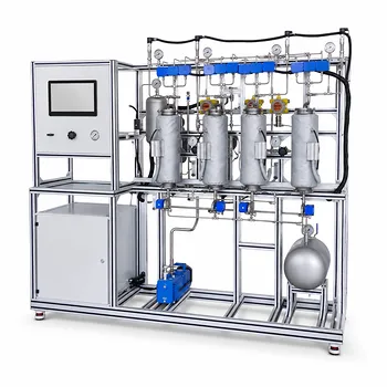
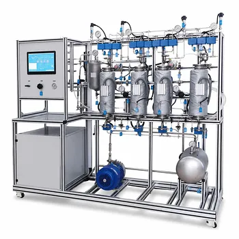
Ready to elevate your chemical engineering labs and research? LABPARK designs and manufactures premium Educational and Vocational Unit Operations Pilot Plants tailored for universities, research institutes, and industrial enterprises. Our state-of-the-art gas absorption pilot plants allow students and researchers to seamlessly validate mass transfer concepts like $N_{OG}$, $H_{OG}$, and column efficiency under precise, real-world conditions.

Chemical Engineering & Bioprocess: High-accuracy pilot columns with inline sensors.
Environmental & Water Treatment: Versatile systems for scrubbing and absorption studies.
Reliable Support: OEM/ODM flexibility and robust construction for long-term educational use.

Contact LABPARK today to request a catalog or custom quote for your laboratory!