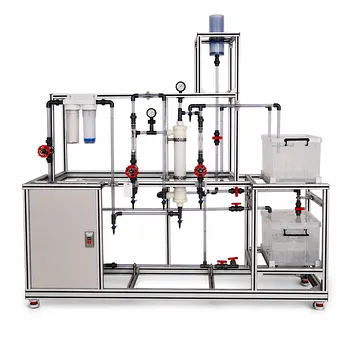
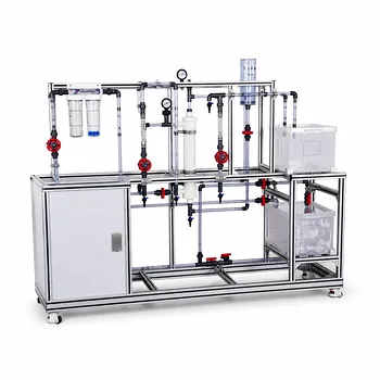
The heart of the lesson is a real-time optical record of molecular binding. In a biotech pilot plant, evanescent wave fiber optic biosensors turn the abstract concept of binding kinetics into a live, quantifiable experiment. Students immobilize antibodies on a quartz fiber core, then flow a fluorescently labeled analyte across it. As binding occurs within the ∼100 nm evanescent field, the fluorescence signal rises in real time. By analyzing the curve’s slope and decay, they directly extract the association rate constant (k₊₁), the dissociation rate constant (k₋₁), and the equilibrium dissociation constant (KD). This single platform, with minor reagent changes, can then demonstrate the same kinetics principles for anything from environmental contaminants to bioremediation bacteria.
The true power for a training pilot plant lies in making kinetics visible and calculable. The evanescent wave biosensor turns a quartz fiber into a transparent kinetic reactor, allowing students to watch binding happen and then critically evaluate the assumptions behind every calculated constant—including how non‑specific binding threatens data integrity and how to control it.
The Physics That Makes It Work
Total Internal Reflection and the Evanescent Field
When laser light travels through an optical fiber by total internal reflection, a tiny fraction of the electromagnetic energy escapes the core. This evanescent wave penetrates roughly 100 nm into the surrounding liquid. It is this shallow excitation zone that gives the biosensor its selectivity.
Why the 100 nm Zone Matters
Only fluorophores within that thin layer are excited. By immobilizing capture antibodies directly on the de‑cladded fiber core, the sensor automatically concentrates the target analyte right at the detection surface. Bulk solution fluorescence contributes almost nothing, so the signal reflects surface binding events with minimal interference.
One Platform, Endless Kinetic Demonstrations
The fiber, light source, and detector stay the same. Only the immobilized recognition element and the fluorescent tracer change. This allows a pilot plant to run back‑to‑back kinetics experiments—antibody‑antigen, DNA hybridization, or bacteria‑antibody—without rebuilding the setup, reinforcing that the kinetic principles are universal.
From Raw Signal to Rate Constants: The Teaching Workflow
Preparing the Sensing Surface
A quartz fiber is stripped of its cladding, cleaned, and coated with a capture antibody. After blocking with a non‑target protein (e.g., casein), the fiber is mounted in a flow cell that allows controlled buffer exchange.
The Association Phase
A solution containing a fluorescently labeled analog of the analyte (often at a concentration as low as 10 nM) is pumped through the flow cell. As the labeled analyte binds to the surface antibodies, the fluorescence intensity climbs. The rising slope gives the apparent association constant (kapp), which under appropriate conditions yields k₊₁.
The Dissociation Phase
Once the signal plateaus, the flow is switched to tracer‑free buffer. The labeled analyte begins to unbind, and the fluorescence decays. The half‑time of dissociation (t₁/₂) directly provides k₋₁.
Calculating the Binding Affinity
With both rate constants in hand, students compute the equilibrium dissociation constant: KD = k₋₁ / k₊₁. Seeing that number emerge from raw optical data makes the link between kinetics and affinity concrete.
Making It Realer: Pilot Plant Applications That Extend the Lesson
Monitoring Bioremediation Bacteria
In a water‑treatment pilot plant, students can immobilize antibodies against a specific dechlorinating bacterium on the fiber. As the bacterial concentration changes in the bioreactor, the real‑time fluorescence generates a kinetic curve that mirrors the earlier antibody‑antigen model. This directly connects kinetics to process control and environmental monitoring.
Detecting Contaminants and Chemical Hazards
Using the same instrument, students can switch reagents to detect trinitrotoluene (TNT) or gram‑negative bacteria. The identical kinetic principles govern the signal rise and fall, teaching that a well‑understood binding mechanism is the foundation of any rapid assay.
The Critical Skills: Understanding and Controlling Non‑Specific Binding
Where Measurement Artifacts Come From
Fluorescent tracers can stick to other proteins (like BSA), the fiber surface itself, or even the flow cell walls. This non‑specific binding adds background that distorts the true kinetic curve, making it look faster or slower than it really is.
Blocking Strategies for a Clean Signal
Pilot‑plant training must show how to manage this. Fibers are pre‑coated with casein or non‑target IgG to block sticky sites. The choice matters: a suboptimal blocker can leave students with a misleading signal‑to‑noise ratio.
Tracer Optimization and Control Fiber Subtraction
Not all fluorescent tracers behave identically. Students can evaluate structurally related tracers to pick the one that gives the highest signal at low concentration (e.g., 10 nM) with the least non‑specific binding. Any residual background is then quantified on a control fiber (coated with irrelevant antibody) and subtracted, making data correction a deliberate analytical step, not an afterthought.
Understanding the Trade-offs and Common Pitfalls
Speed vs. Label Interference
The fluorescent label itself can alter the analyte’s binding kinetics. Introducing a tracer that behaves identically to the unlabeled target is an assumption that must be tested, and this tension becomes a powerful teaching point about label‑free vs. label‑based methods.
Surface Regeneration Limits Throughput
Between experiments, the antibody layer must be gently regenerated (e.g., with a mild acid pulse) to strip the bound analyte without destroying activity. Reproducibility across regeneration cycles is not guaranteed, and students quickly learn that a poorly regenerated fiber gives misleading rate constants.
The 100 nm Window Blindness
The evanescent field only reports events at the very surface. Mass transport limitations or aggregation in the bulk can mean the surface concentration does not accurately reflect the bulk concentration, introducing errors in kapp if the flow rate is not optimized.
Making the Right Choice for Your Training Pilot Plant
After a brief discussion on goals, use these specific recommendations.
- If your primary focus is teaching fundamental binding kinetics: Anchor the exercise on a simple antibody‑antigen pair with a well‑characterized fluorescent tracer. Focus on manual extraction of k₊₁ and k₋₁ from the raw data, and have students justify every assumption in the KD calculation.
- If your primary focus is bioprocess monitoring and quality control: Extend the core kinetics experiment into a practical assay for a real‑world target (e.g., a contaminant or a process‑critical bacteria). Emphasize tracer selection, blocking protocols, and control‑fiber subtraction as the keys to reproducible data.
- If your primary focus is instrument design or vocational training: Keep the optical platform constant and rotate multiple analyte‑reagent systems. Use the unchanged hardware to highlight that reliable kinetic measurements are 90% about surface chemistry and flow control, not about the sensor itself.
Once students see a binding curve resolve into two numbers and a KD, they’ve moved beyond theory—they’ve become operators who can diagnose sensor performance and understand what a “good” kinetic constant really means.
Summary Table:
| Phase | Key Action | Measured Parameter |
|---|---|---|
| Preparation | Immobilize antibody & block with casein | Surface baseline stability |
| Association | Flow fluorescent analyte (10 nM) | Association rate constant ($k_{+1}$) |
| Dissociation | Flow tracer-free buffer | Dissociation rate constant ($k_{-1}$) |
| Analysis | Compute $K_D = k_{-1} / k_{+1}$ | Equilibrium dissociation constant ($K_D$) |
Bring Advanced Biotech Kinetics to Your Lab
Hands-on training with real-time biosensors prepares students for modern bioprocess challenges. LABPARK provides premium Educational and Vocational Unit Operations Pilot Plants in chemical engineering, bioprocess & biotech, and environmental & water treatment. We help universities, research institutes, and enterprises build practical, industry-ready skills.
Contact LABPARK today to discover how our custom pilot plants can transform your training programs!
Related Products
- Cavitation Phenomenon Demonstration and Analysis Educational Unit Operations Pilot Plant
- Multifunctional Membrane Separation Educational Pilot Plant with Ultrafiltration, Nanofiltration, Reverse Osmosis
- Orifice and Venturi Flowmeter Calibration Educational Pilot Plant for Fluid Mechanics Laboratory
- Ultrafiltration Membrane Separation Educational Pilot Plant
- Fluid Friction Resistance Determination Educational Unit Operations Pilot Plant
People Also Ask
- How do pilot plants teach U-tube manometers? Master Differential Pressure Calculations
- How to teach pump cavitation vs. gas binding? Interactive pilot plant teaching guide.
- What factors should be considered when selecting float valve types? F1 vs. V-4 vs. T-type Guide
- How does an FIA biosensor improve fermentation monitoring compared to HPLC? Speed & automation.
- What are key parameters for stable biosensor FIA in bioprocess training? Achieve optimal performance.