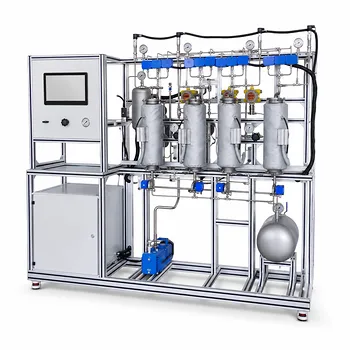
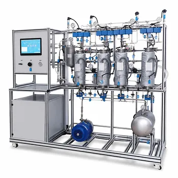
How To Determine Kya In A Gas Absorption Pilot Plant? A Practical Guide

The direct answer is straightforward. To experimentally determine the volumetric overall mass transfer coefficient ($K_Y a$) in a gas absorption pilot plant, you operate the column at steady state, measure inlet and outlet solute concentrations in both the gas and liquid phases, and know the gas and liquid flow rates. From these, you perform a material balance to calculate the total solute absorption rate ($G_A$), evaluate the log‑mean driving force ($\Delta Y_m$) using the equilibrium relationship, and divide $G_A$ by the product of the packed bed volume ($V_p$) and $\Delta Y_m$. This yields $K_Y a$, the lumped parameter that quantifies how fast the solute moves from the gas into the liquid per unit volume of packing.

Understanding $K_Y a$ experimentally turns a complex mass transfer theory into a practical design tool. The real goal is not just plugging numbers into a formula—it’s learning to control operating conditions, correctly evaluate the true driving force, and assess the reliability of the result. This transforms a pilot‑plant run from a simple measurement into a validation of the underlying principles that govern industrial absorption columns.

Why This Experiment Matters More Than the Number Itself

It Connects Theory to a Tangible Column Performance

Chemical engineering textbooks present $K_Y a$ as a key design parameter. Running an absorption pilot plant lets you see that this coefficient is not a constant but a function of hydrodynamics, packing type, and system properties. The experiment forces you to confront the real‑world interplay between thermodynamics (equilibrium) and rate processes (mass transfer).

It Teaches You How to Judge Your Own Data

A single $K_Y a$ value has limited worth unless you know the uncertainty in your concentration measurements, whether the column actually reached steady state, and if the driving force was correctly expressed. The pilot plant becomes a laboratory for critical data evaluation.

Step‑by‑Step Experimental Determination of $K_Y a$

What You Must Measure Before Starting the Calculation

First, establish steady‑state conditions. The outlet concentrations of the solute in both the gas and liquid streams must be stable for at least several residence times. Record:

Gas flow rate (molar or volumetric basis, converted to inert‑free or carrier‑gas flow if needed).
Liquid flow rate.
Solute mole fractions (or mass ratios) at the gas inlet ($Y_{A,in}$) and outlet ($Y_{A,out}$).
Solute concentrations in the liquid at the inlet ($X_{A,in}$) and outlet ($X_{A,out}$).

Performing the Material Balance to Find $G_A$

The rate of solute transfer from the gas to the liquid, $G_A$, is obtained from the change in the gas‑phase solute flow between inlet and outlet. If $G_s$ is the molar flow rate of the inert carrier gas (constant along the column), then: $G_A = G_s (Y_{A,in} - Y_{A,out})$

If the liquid‑phase balance is used instead, $G_A = L_s (X_{A,out} - X_{A,in})$, where $L_s$ is the inert liquid flow rate. Discrepancies between the two balances reveal measurement errors and must be reconciled before proceeding.

Determining the Packed Bed Volume ($V_p$)

$V_p$ is often a fixed geometric property of the pilot plant. Measure the column’s internal diameter and the height of the packed section (from the support plate to the top of the packing). $V_p = \text{cross‑sectional area} \times \text{packed height}$. For modular columns, verify that the packing is seated uniformly.

Calculating the Driving Force ($\Delta Y_m$) Correctly

The driving force for the gas‑phase overall coefficient is $\Delta Y = Y_A - Y_A^$, where $Y_A^$ is the gas‑phase mole ratio in equilibrium with the bulk liquid composition at that horizontal slice of the column. Because both operating and equilibrium lines are typically curved, the log‑mean driving force is used:

$\Delta Y_m = \frac{(Y_{A,in} - Y_A^{out}) - (Y_{A,out} - Y_A^{in})}{\ln\left(\frac{Y_{A,in} - Y_A^{out}}{Y_{A,out} - Y_A^{in}}\right)}$

$Y_A^*{out}$ is the gas‑phase mole ratio in equilibrium with the exiting liquid ($X_{A,out}$).
$Y_A^*{in}$ is the gas‑phase mole ratio in equilibrium with the entering liquid ($X_{A,in}$).

If the equilibrium relationship follows Henry’s law, $Y_A^* = m X_A$, where $m$ is the Henry’s law constant expressed in suitable units (e.g., mole ratio/mole ratio). Determine $m$ from literature or a separate equilibrium measurement at the column’s operating temperature and pressure.

Assembling the Final Formula

Once $G_A$, $V_p$, and $\Delta Y_m$ are known, calculate:

$K_Y a = \frac{G_A}{V_p , \Delta Y_m}$

The result has units of moles transferred per unit time, per unit packing volume, per unit driving force (e.g., $\mathrm{kmol/(m^3 \cdot s \cdot \Delta Y)}$). This single number encapsulates both the overall mass transfer coefficient ($K_Y$) and the effective interfacial area per unit volume ($a$), both of which are influenced by flow rates and packing geometry.

Understanding the Trade‑offs and Common Pitfalls

The Danger of Assuming a Linear Equilibrium Throughout the Column

If the equilibrium line is significantly curved, the simple log‑mean expression overestimates or underestimates the true driving force. You may need to use a graphical or numerical integration (the “NTU‑HTU” method) instead of a single $\Delta Y_m$. The primary reference formula is exact only for a linear equilibrium relationship and dilute systems where mole ratios and mole fractions are interchangeable.

Steady‑State Is Deceptively Hard to Recognize

Concentration profiles can take much longer to stabilize than you expect, especially if the liquid holdup is large. A premature reading will give a $K_Y a$ that does not reflect the true column performance. Always take at least three consecutive sets of consistent readings over a span of 10–15 minutes.

The Material Balance Must Close

When the $G_A$ calculated from the gas side does not match the liquid side within about 5–10%, do not trust the $K_Y a$. The mismatch often arises from solute loss to the environment, sampling errors, or inaccurate flow meters. Investigate the discrepancy before interpreting the result.

$K_Y a$ Is Not an Intrinsic Property

Remember that $K_Y a$ changes with liquid and gas flow rates, packing type, and system chemistry. A value measured at one set of conditions cannot be blindly applied to a different operating point. The experiment’s real educational value is in mapping how $K_Y a$ varies with liquid and gas velocities—this is the basis for scale‑up.

Making This Experiment Work for Your Learning or Research Goal

If your primary focus is mastering mass transfer fundamentals: Start by verifying that the equilibrium relationship you use (Henry’s constant) is accurate for your system and temperature. Then, replicate the experiment at three different gas flow rates and observe how $K_Y a$ increases, linking that change to turbulence and interfacial area.
If your primary focus is obtaining reliable design data: Rigorously close the material balance every time and report a confidence interval for $K_Y a$ based on propagated measurement uncertainties. Compare your value with published correlations for the same packing to validate your procedure.
If your primary focus is understanding column hydrodynamics: Measure the pressure drop across the packing simultaneously and note the onset of loading and flooding. Relate these hydrodynamic signatures to abrupt changes in $K_Y a$, showing how mass transfer performance degrades outside the optimal operating window.

When you treat the pilot plant not as a black box that outputs a number, but as a system that reveals the physics of interphase transport, the calculated $K_Y a$ becomes a reliable foundation for everything from scale‑up to troubleshooting.

Summary Table:

Step	Action / Parameter	Formula & Key Consideration
1. Steady State Data	Measure flow rates & compositions	Ensure stable inlet/outlet compositions ($Y_{in}, Y_{out}, X_{in}, X_{out}$)
2. Solute Transfer Rate	Calculate solute absorbed ($G_A$)	$G_A = G_s(Y_{in} - Y_{out})$
3. Driving Force	Calculate log-mean driving force	$\Delta Y_m = \frac{(Y_{in} - Y^{out}) - (Y{out} - Y^{in})}{\ln[(Y{in} - Y^{out}) / (Y{out} - Y^_{in})]}$
4. Mass Transfer Coeff.	Solve for overall coefficient	$K_Y a = \frac{G_A}{V_p \Delta Y_m}$

Ready to elevate your practical training and laboratory research? LABPARK provides state-of-the-art Educational and Vocational Unit Operations Pilot Plants in chemical engineering, bioprocess & biotech, and environmental & water treatment. Built specifically for universities, research institutes, and enterprises, our equipment bridges the gap between complex mass transfer theory and hands-on application. Contact us today to find the perfect pilot plant solution for your institution!