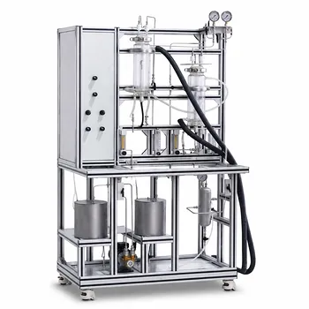
Step input tracer experiments minimize systematic measurement errors, directly provide the cumulative distribution function without numerical manipulation, and instantly reveal flow anomalies through simple visual inspection. These practical advantages make them a more robust and reliable choice for analyzing reactor dynamics in a unit operations teaching pilot plant, where clear, accurate data is essential for student learning and experimental diagnostics.
While pulse injections are intuitive and widely used in teaching labs, step input experiments offer superior accuracy and simplicity for the core analytical goals of a pilot plant. By canceling instrument bias, yielding the F(t) curve directly, and allowing immediate detection of maldistributions without complex math, they reduce experimental uncertainty and make reactor behavior instantly comprehensible.
The Practical Advantages of Step Input Tracer Experiments
The preference for step input experiments in a teaching pilot plant stems from three concrete, error-reducing features that align perfectly with the educational and diagnostic goals of unit operations labs.
Instrument Bias Cancellation
The most overlooked source of inaccuracy in tracer studies is systematic measurement error.
In a step experiment, the same analytical instrument (e.g., a conductivity cell or spectrophotometer) measures both the inlet feed concentration and the outlet concentration. Because the key metric is the ratio ( C(t)/C_f ), any consistent calibration offset or drift cancels out. This is not the case for a pulse injection, where the absolute outlet concentration ( C(t) ) must be compared to the known injected mass ( m ); any instrument bias directly corrupts the calculated ( E(t) ) curve.
Direct Measurement of F(t) and Escape Probability
Step input eliminates the single largest mathematical pitfall of pulse experiments: numerical differentiation.
A step change immediately gives you the cumulative distribution function, ( F(t) ), as the normalized outlet response. The complement, ( 1-F(t) ), which is the fraction of fluid that has spent at least time ( t ) in the reactor, can then be plotted directly. From this, the escape probability (intensity function) is computed with simple algebra—no integration or differentiation is required. Pulse experiments, by contrast, yield the density function ( f(t) ) directly, but any subsequent calculation of ( F(t) ) or related diagnostics involves numerical integration that amplifies baseline noise and injection-tail errors.
Immediate Visualization of Flow Maldistributions
Step response curves speak a visual language that requires no interpretation filter.
A properly functioning reactor with regular flow will produce a smooth, monotonic step response rising from zero to one. Any deviation—such as a temporary dip, a plateau, or an overshoot—is immediately visible on the chart recorder or data screen. These non-monotonic features flag bypassing, stagnant zones, flow rate fluctuations, or turbulent mixing the moment they occur, without the need to fit a model or back-calculate distributions. In a teaching environment, this real-time diagnostic ability accelerates learning and troubleshooting.
How Step Input Differs from Pulse Input in a Teaching Lab
Pulse injections feel straightforward: shoot a slug of tracer and watch it emerge. But their apparent simplicity hides several layers of experimental fragility that become magnified in a pilot plant setting.
The Sensitivity of Pulse Injections
A pulse experiment requires that the tracer be injected instantaneously—in a timeframe that is negligible relative to the mean residence time of the reactor. Any finite injection duration, imperfect mixing at the inlet, or tailing from injection hardware creates an input signal that is not a true Dirac delta function, distorting the measured ( f(t) ). Furthermore, the denominator in the calculation, the total tracer mass ( m ), must be known exactly; even a small weighing or volumetric error propagates directly into the shape of the residence-time distribution.
Educational Context: Reliability Over Intuition
While students often find the “peak-and-tail” of a pulse experiment intuitive, that intuition can be misleading. A pulse curve’s shape is highly sensitive to both injection technique and downstream integration choices. In contrast, the step method, despite requiring a larger tracer volume, is far easier to execute consistently. There is no critical injection time window; you simply switch a valve. The result is data that is inherently more repeatable and less dependent on operator skill—exactly what you want in a teaching pilot plant where multiple student groups will run the same experiment.
Understanding the Trade-offs
No method is universally superior. Step input experiments come with their own costs, and it’s important to acknowledge when a pulse might still be the better tactical choice.
The Resource Trade-off
Step experiments consume a larger volume of tracer fluid because the feed must be switched over for a sustained period until the outlet concentration reaches steady state. In a large pilot-scale reactor, this may involve significant chemical cost and waste disposal. However, for typical educational pilot plants (which are smaller in scale), this volume is rarely prohibitive, especially when weighed against the quality of the data obtained.
When Pulse Experiments Still Shine
Pulse injections remain valuable when tracer material is extremely expensive, in very large industrial reactors where a step change would require prohibitive amounts, or when the reactor’s inlet configuration allows a near-perfect instantaneous injection. They also naturally yield the ( f(t) ) curve, which can be more directly related to fundamental dispersion models. So the preference for step input is not a dismissal of the pulse method, but a pragmatic decision based on typical teaching pilot plant constraints and learning objectives.
Making the Right Choice for Your Teaching Pilot Plant
Align your tracer method with the specific learning outcomes and operational realities of your unit operations lab.
- If your primary focus is minimizing measurement uncertainty and data scatter: Choose a step input experiment. Instrument bias cancellation and direct ( F(t) ) extraction remove the two largest sources of error.
- If your primary focus is rapid, visual diagnosis of reactor flow problems: Use a step input. Non-monotonic step responses immediately flag bypassing, dead zones, or unstable flow without any post-processing.
- If your primary focus is demonstrating the fundamental concept of the residence-time density function directly: A pulse experiment may be more pedagogically direct for that single concept, but be prepared to invest significant time in injection technique and error analysis.
- If your primary focus is running a high-throughput lab with multiple student teams and limited instructor oversight: Lean heavily on step experiments. Their repeatability and ease of execution ensure that differences between groups reflect real reactor behavior, not operator variability.
The goal of a unit operations pilot plant is to transform abstract residence-time theory into undeniable, visual truth. Step input tracer experiments give you the clearest lens to make that happen.
Summary Table:
| Feature | Step Input Experiment | Pulse Input Experiment |
|---|---|---|
| Calibration Offset | Cancels out automatically ($C(t)/C_f$ ratio) | Directly corrupts results ($C(t)$ vs. mass $m$) |
| Mathematical Pitfalls | None (direct $F(t)$ measurement) | Requires integration (amplifies baseline noise) |
| Flow Maldistributions | Instantly visible on chart recorder | Requires post-processing / model fitting |
| Execution Complexity | Low (simple valve switch, highly repeatable) | High (requires instant injection and exact mass) |
| Tracer Consumed | High volume (sustained feed) | Low volume (single slug) |
Enhance your student learning outcomes and experiment accuracy with state-of-the-art training systems. LABPARK provides premium Educational and Vocational Unit Operations Pilot Plants in chemical engineering, bioprocess & biotech, and environmental & water treatment for universities, research institutes, and enterprises.
Need help configuring the ideal reactor dynamics setup for your laboratory? Contact our expert team today to receive a customized solution tailored to your curriculum and research goals!
Related Products
- Multi Functional Catalytic Reaction and Reactor Evaluation Educational Unit Operations Pilot Plant
- Residence Time Distribution and Reactor Flow Characteristics Determination Educational Pilot Plant
- Tubular Reactor Flow Characteristics Determination Educational Unit Operations Pilot Plant
- 100L Continuous Loop Hydrogenation Educational Unit Operations Pilot Plant
- Multi-Stage Stirred Tanks in Series Residence Time Distribution and Mixing Performance Determination Educational Pilot Plant
People Also Ask
- What reaction engineering principles are shown in a catalytic reactor pilot plant? SO2 Oxidation Guide
- How does feed gas flow rate affect catalytic RFR yields? Optimize Pilot Plant Performance
- Why is FTIR integration in catalytic pilot plants important? Real-Time Student Insights
- How to analyze active metal distribution & identify catalyst poisoning in pilot plants? Expert Diagnostic Guide
- How to study catalyst poisoning & regeneration? Master catalytic reaction life cycles.