How To Simplify Low-Pressure Solubility To Vle Conversion? Boost Pilot Plant Efficiency.

The key to simplification lies in the ideal gas assumption. When running gas absorption or distillation pilot plants at low pressure, you can immediately set the vapor fugacity coefficient to 1.0. This collapses the full equilibrium constant to K = γ f_L° / π, letting you convert standard solubility data (like Bunsen or Ostwald coefficients) directly into usable activity coefficients without any high-pressure equation of state.

Pilot‑plant engineers simplify low‑pressure VLE conversion by treating the vapor phase as ideal. That single step eliminates complex fugacity corrections, reduces the K‑value to a clean function of activity coefficient and system pressure, and lets you back‑calculate γ from solubility measurements—providing a fast, reliable correlation that bridges the gap between lab data and column operation.

The Thermodynamic Shortcut for Low‑Pressure VLE

The rigorous K‑value expression includes vapor‑phase non‑ideality, but at pressures near 1 atm those terms become negligible. Understanding which pieces fall away gives you a rule‑of‑thumb that is both mathematically sound and operationally safe.

Stripping Down the Rigorous K‑Value Expression

The full VLE relationship equates the partial fugacity of a component in both phases. At low pressure, the vapor phase is essentially an ideal gas: the vapor mole fraction yᵢ can be treated as 1.0 and the fugacity coefficient φᵢ = 1.0.

With those assumptions eliminated, the equilibrium constant reduces to the ratio you will actually use in the plant: K = γ f_L° / π. Here γ is the liquid‑phase activity coefficient, f_L° is the standard‑state liquid fugacity, and π is the total system pressure.

System pressure is measured directly on the pilot‑plant control panel. The challenge shifts entirely to finding γ and f_L° from your solubility data.

From Solubility Measurements to Activity Coefficients

Standard solubility experiments report how much gas dissolves in a liquid at a known temperature and partial pressure. In a low‑pressure pilot plant, those measurements are the raw material for building your K‑value correlations.

You can invert the simplified K‑value equation to solve for the activity coefficient. If you already know f_L° — often approximated by the pure‑component vapor pressure for subcritical species or by a Henry’s law constant for a supercritical gas — the only unknown is γ.

Once γ is extracted, it becomes a function of temperature and liquid composition. This is the thermodynamic fingerprint you will feed into your column model, whether you are running a simple batch distillation or a continuous absorption loop.

Translating Standard Solubility Data into K‑Values

The practical conversion pipeline runs from a solubility measurement to a temperature‑dependent correlation you can load into a distributed control system or a steady‑state simulator.

Using Bunsen and Ostwald Coefficients

Bunsen and Ostwald coefficients are direct measures of gas solubility: they tell you the volume of gas dissolved per volume of liquid at a reference condition. Both are standard outputs from low‑pressure solubility experiments.

For the Bunsen coefficient, the measurement is taken at a known partial pressure and temperature. By converting the dissolved volume to a liquid mole fraction x, you can calculate the equilibrium K‑value as K = y/x, where y is the vapor mole fraction at that same partial pressure (effectively y = p_partial / π).

The Ostwald coefficient gives a similar path but is defined on a volume‑ratio basis. In either case, the operation is simple arithmetic because the ideal‑gas assumption lets you treat p_partial and y as linearly related.

Building T‑Dependent Correlations

Solubility is strongly temperature‑dependent, so a single data point at one temperature is rarely enough. Pilot‑plant teams typically collect solubility data at 3‑5 temperatures spanning the column’s expected operating range.

From each measurement you extract γ, then fit the log of γ against 1/T using a two‑ or three‑parameter correlation. This captures the temperature behavior needed to predict K‑values at any tray or packing section where the liquid temperature differs from the reboiler or condenser.

A robust correlation means you can run the pilot plant without repeatedly re‑measuring solubility, yet still account for the natural temperature profile inside the column.

Understanding the Trade‑offs and Limitations

Every simplification carries risk. The ideal‑gas shortcut works beautifully in its intended window, but blind use outside that window will compromise both safety and separation efficiency.

The Pitfall of Extrapolating to Higher Pressures

Most standard VLE data is recorded at 1 atm, yet industrial columns often operate up to 15 atm to improve energy integration. The moment you pressurize a pilot plant, the ideal‑gas assumption cracks.

At elevated pressure, vapor‑phase non‑ideality returns with force. Fugacity coefficients can deviate significantly from 1.0, and neglecting them gives K‑values that are dangerously optimistic or pessimistic. The simplified equation γᵢ xᵢ pᵢˢᵃᵗ = yᵢ P — so popular in undergraduate textbooks — becomes invalid the instant a component operates above its critical temperature or the pressure passes roughly 5 atm.

Continuing to use the low‑pressure shortcut in a high‑pressure column can lead to massive over‑design (too many stages, oversized boilers) or, worse, an under‑designed column that fails to meet purity specs.

When Non‑Ideal Liquid Phases Break the Model

Even at low pressure, the liquid phase can exhibit strong non‑ideality — for example, in systems with hydrogen bonding, electrolytes, or significant size differences between molecules. In those cases, the activity coefficient γ itself becomes complex.

The K = γ f_L° / π form is still valid, but γ can no longer be treated as a simple temperature‑only function. Sudden composition‑dependent excursions can occur, and your correlation might miss azeotropic or near‑azeotropic behavior unless you explicitly measure composition‑dependent data.

A pure temperature correlation might give you excellent fits at one liquid composition but fail badly when the pilot plant deviates from that baseline — such as during startup, upset conditions, or when processing a mixed feed.

The Over‑Design Trap: Learning from Shortcut History

Historically, process designers used short‑cut methods like Fenske‑Underwood‑Gilliland because rigorous VLE data was scarce. The result was systematic over‑design: columns with extra stages, oversized reboilers, and conservatively high reflux ratios.

While that safety margin prevented disasters, it also inflated capital and operating costs. By using a low‑pressure pilot plant to directly measure γ and build a proper K‑value correlation, you can reverse that habit and design closer to the thermodynamic optimum, saving energy in the reboiler and condensation load in the condenser.

Scaling Up: Bridging Low‑Pressure Data to Industrial Conditions

The low‑pressure pilot plant is the launch pad; the full‑scale industrial column is the target. The bridge is built by combining your γ correlations with a proper equation of state.

Integrating an Equation of State for φᵢ

When you move to elevated pressures, the K‑value must be restored to its full form: K = (γ f_L°) / (φᵢ π). The γ you obtained from low‑pressure solubility data remains valid — it is a liquid‑phase property largely independent of pressure.

The vapor‑phase fugacity coefficient φᵢ is calculated from an equation of state like Peng‑Robinson or Soave‑Redlich‑Kwong. An iterative loop updates φᵢ with the predicted vapor composition until convergence.

Pilot plants that allow pressurized operation are invaluable here. They let you switch from the low‑pressure ideal‑gas regime to a high‑pressure real‑gas regime, measuring actual partial pressures as a function of temperature and concentration to verify that your φᵢ predictions hold.

Validating with Pilot Plant Measurements

No simulation can replace experimental data when complex chemical‑physical interactions are at play — acid gas scrubbing is a classic example. Thermodynamics can extend the utility of experimental data, but it cannot substitute for it.

Taking physical samples of both phases at stabilized temperature and pressure directly confirms whether the system has reached true phase equilibrium, and whether the K‑values derived from low‑pressure solubility correctly map to the real plant.

These measurements give you the binary group interaction parameters (e.g., for NRTL or UNIQUAC models) that make process simulators trustworthy, enabling confident scale‑up under the exact conditions the full‑scale unit will face.

Making the Right Choice for Your Pilot Plant Goal

Your decision tree depends on what you need the pilot plant to answer. Use these goal‑based recommendations to select the right level of thermodynamic complexity.

If your primary focus is quick screening at atmospheric pressure: Rely on the ideal‑gas simplification K = γ f_L° / π, and build γ correlations directly from Bunsen or Ostwald solubility data. This keeps your operation fast and your data processing simple.
If your primary focus is generating scale‑up data for a pressurized industrial column: Start with the low‑pressure γ correlations, then layer in an equation‑of‑state calculation for φᵢ to extend the model to higher pressures, and validate with physical samples at the elevated conditions.
If your primary focus is minimizing over‑design and energy cost: Reject historical short‑cut methods. Use the pilot plant to measure composition‑ and temperature‑dependent γ from solubility data, and build a precise K‑value model that supports tight column sizing and lower reflux ratios.

The power of the low‑pressure solubility shortcut is that it transforms a formidable thermodynamic problem into a clean, manageable correlation exercise — giving you accurate K‑values for your pilot plant today and a firm foundation for the industrial design of tomorrow.

Summary Table:

Parameter	Low-Pressure VLE (< 5 atm)	High-Pressure VLE (> 5 atm)
Vapor Phase Assumption	Ideal Gas (phi_i ≈ 1.0)	Real Gas (Requires Equation of State)
Simplified K-Value Equation	K = γ * f_L° / π	K = γ * f_L° / (phi_i * π)
Primary Challenge	Finding liquid-phase activity (γ)	Calculating phi_i and composition dependence
Application	Atmospheric distillation & absorption	Industrial scale-up & pressurized columns

Optimize Your Chemical Engineering Lab with LABPARK

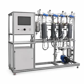
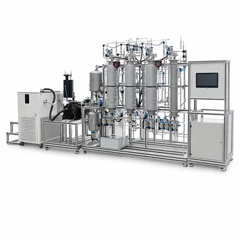
Scaling up distillation and absorption processes requires reliable thermodynamic data and robust equipment. LABPARK provides state-of-the-art Educational and Vocational Unit Operations Pilot Plants in chemical engineering, bioprocess & biotech, and environmental & water treatment.

Designed specifically for universities, research institutes, and enterprises, our pilot plants deliver the precision, safety, and control you need to validate thermodynamic models, run scale-up simulations, and train the next generation of engineers.

Ready to elevate your research and training capabilities? Contact us today to discuss your custom pilot plant needs!