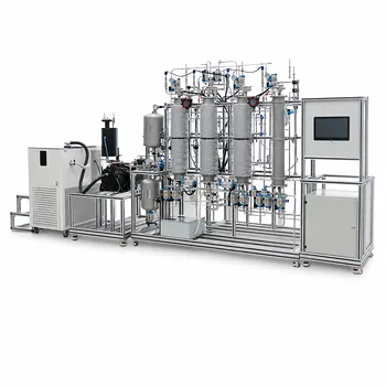
During the initial stage of operation, treat the membrane as a semi-infinite slab rather than a finite layer. If the elapsed time is short enough that the penetration depth (\delta(t) \approx \sqrt{Dt}) remains much smaller than the membrane thickness (L), solute has not reached the opposite interface. The external feed can then be treated as a constant-concentration reservoir, allowing the membrane diffusion problem to be solved independently of the coupled external mass balances.

For early-time membrane operation, replace the finite membrane domain with a semi-infinite one and hold the feed concentration at its initial value. This converts the coupled pilot-plant problem into a standard transient Fickian diffusion problem, typically represented by an error-function concentration profile.

Why the Full Coupling Can Be Simplified

The source of the coupling

In a complete membrane model, solute concentration changes inside the membrane are coupled to differential balances in the external feed and permeate compartments. As solute leaves or enters those compartments, their concentrations change, which in turn changes the membrane boundary conditions.

This requires solving the membrane diffusion equation together with time-dependent external volume balances.

The short-time condition

Immediately after a step change in feed concentration, solute penetrates only a shallow region near the membrane surface. The characteristic penetration depth is

[ \delta(t) \approx \sqrt{Dt} ]

where (D) is the solute diffusion coefficient in the membrane and (t) is elapsed time.

The semi-infinite approximation is appropriate when

[ \delta(t) \ll L ]

or, equivalently,

[ t \ll \frac{L^2}{D} ]

The quantity (L^2/D) is the characteristic diffusion time required for solute to traverse the membrane.

How to Formulate the Simplified Model

Hold the feed concentration constant

If the external feed volume is sufficiently large relative to the amount transferred during the initial period, its concentration can be approximated as constant:

[ C_1(0,t) \approx C_0 ]

This removes the need to calculate the instantaneous feed concentration from an external differential mass balance.

Replace the finite domain with a semi-infinite domain

Instead of solving across (0 \leq x \leq L), solve the diffusion equation over (x \geq 0):

[ \frac{\partial C}{\partial t}

D\frac{\partial^2 C}{\partial x^2} ]

The unpenetrated region is treated as effectively infinitely far away, so its concentration remains at its initial value:

[ C(\infty,t)=0 ]

This is valid because the concentration disturbance has not yet traveled across the actual membrane thickness.

Use the error-function solution

For a step change at the membrane surface, the transient profile has the standard form

[ \frac{C(x,t)-C_{\text{initial}}} {C_{\text{surface}}-C_{\text{initial}}}

\operatorname{erfc} \left( \frac{x}{\sqrt{4Dt}} \right) ]

depending on the chosen initial and boundary concentration convention. An equivalent formulation uses the error function:

[ \frac{C(x,t)-C_{\text{surface}}} {C_{\text{initial}}-C_{\text{surface}}}

\operatorname{erf} \left( \frac{x}{\sqrt{4Dt}} \right) ]

These expressions provide the concentration profile without numerically integrating the external reservoir balances.

What This Approximation Provides

Initial transient flux

The surface flux can be obtained directly from Fick’s first law:

[ J(t)=-D\left.\frac{\partial C}{\partial x}\right|_{x=0} ]

For a step change into an initially solute-free membrane, the magnitude of the flux is proportional to

[ J(t)\propto \left(C_{\text{surface}}-C_{\text{initial}}\right) \sqrt{\frac{D}{t}} ]

Thus, the initial flux is high and decreases with time as the concentration disturbance spreads into the membrane.

Early-stage concentration profiles

The solution estimates how far solute has traveled and how sharply the concentration changes near the feed interface. This is useful for interpreting startup data and identifying whether a measured response is still controlled by membrane penetration.

A practical diagnostic model

The semi-infinite solution can serve as a quick benchmark for pilot-plant data. If the measured response agrees with the predicted early-time behavior, the membrane is likely still in the penetration-controlled regime.

Significant deviation may indicate that the membrane has reached the opposite interface, the feed concentration is no longer constant, or additional mechanisms such as convection, partitioning, or reaction are important.

When the Approximation Stops Being Valid

Penetration approaches the membrane thickness

Once

[ \delta(t) \sim L ]

the solute has begun to sense the far side of the membrane. The semi-infinite assumption then becomes inaccurate, and a finite-slab model with a boundary condition at (x=L) is required.

The external reservoir is not large enough

If substantial solute transfer changes the feed concentration, the boundary condition (C_1(0,t)=C_0) is no longer reliable. The external mass balance must then be coupled to the membrane transport equation.

The process approaches steady state

At long times, the membrane moves toward thin-film or finite-slab behavior. The concentration profile is then governed by both membrane thickness and the conditions at both interfaces, rather than by the early-time error-function solution alone.

Understanding the Trade-offs

Main benefit

The approximation reduces a coupled dynamic problem to a single transient diffusion equation. This makes hand calculations, parameter estimation, and early pilot-plant diagnosis substantially simpler.

Main limitation

It does not predict the complete concentration history of the external compartments. It is an initial-period approximation, not a replacement for the full model when reservoir depletion or cross-membrane equilibration becomes important.

Common modeling mistake

The condition (t \ll L^2/D) should be checked using the relevant membrane thickness and diffusion coefficient. Applying the semi-infinite model merely because the experiment has just started can produce incorrect fluxes if the membrane is very thin or diffusion is very fast.

Interface properties still matter

If the solute partitions between the external liquid and the membrane, the membrane-side surface concentration may not equal the liquid-phase concentration. A partition coefficient (H) may therefore be required to relate the boundary concentrations, even when the external balances are temporarily neglected.

Making the Right Choice for Your Goal

Use the following criteria before applying the simplified model:

If your primary focus is initial transient behavior: Use the semi-infinite slab approximation with (\delta(t)\approx\sqrt{Dt}) and an error-function concentration profile.
If your primary focus is startup flux: Treat the feed as a constant-concentration reservoir and calculate the surface flux from the transient diffusion gradient.
If your primary focus is full batch or compartment dynamics: Couple the membrane equation to the external volume balances once reservoir concentrations change appreciably.
If your primary focus is steady-state performance: Use a finite-thickness membrane model with boundary conditions at both interfaces after the diffusion time (L^2/D) has been reached.

By comparing the penetration depth with the membrane thickness and the amount transferred with the external reservoir inventory, you can determine when the simplified transient model is technically justified.

Summary Table:

Modeling aspect	Simplified approach	Validity criterion or benefit
Membrane domain	Treat the membrane as a semi-infinite slab	Penetration depth (\sqrt{Dt}) is much smaller than thickness (L)
Feed boundary	Hold feed concentration at its initial value	External reservoir is large and concentration change is negligible
Governing model	Solve transient Fickian diffusion independently	Avoids fully coupled external mass-balance equations
Concentration profile	Use an error-function or complementary error-function solution	Estimates early-stage solute penetration
Startup flux	Calculate flux from the transient concentration gradient	Flux typically decreases in proportion to (t^{-1/2})
Model limit	Switch to a finite-slab coupled model	Required when (t) approaches (L^2/D) or reservoir depletion becomes significant

Need reliable membrane separation training or pilot-scale data for your next project? Contact LABPARK to discuss Educational and Vocational Unit Operations Pilot Plants for chemical engineering, bioprocess and biotech, and environmental and water treatment applications. LABPARK helps universities, research institutes, and enterprises evaluate transient membrane behavior, demonstrate transport principles, train students and operators, and build practical process-development capabilities with equipment designed for clear observation, repeatable experiments, and effective technical education.