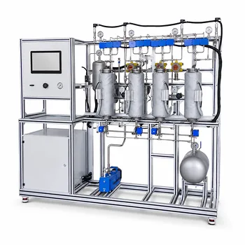
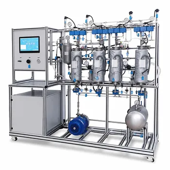
How Countercurrent Flow In Absorption Columns Optimizes Mass Transfer For Lab Training: A Practical Guide.

The defining feature of an absorption column pilot plant is its countercurrent flow design. By feeding the liquid solvent at the top and the gas mixture at the bottom, the column maintains a persistently high concentration gradient between the two phases over its entire height. This physical arrangement maximizes mass transfer efficiency, ensuring the leanest gas contacts the freshest solvent at the column’s top while the richest gas meets the solvent loaded with solute at the bottom. For laboratory training, this setup allows participants to directly observe gas purification, gather experimental data, and calculate material balances and absorption kinetics in a controlled, hands-on environment.

The countercurrent flow design is the engine of an absorption column’s efficiency: it sustains a high and uniform mass transfer driving force from top to bottom, which lowers the outlet gas’s solute concentration, reduces solvent usage, and creates an ideal, transparent setup for students to quantify and optimize gas-liquid mass transfer.

How the Countercurrent Flow Maximizes the Driving Force

The Physics of a Perpetual Gradient

Mass transfer from gas to liquid is driven by the difference in solute concentration between the two phases. In a countercurrent column, the gas that rises with the lowest remaining solute concentration is met by the purest solvent descending from the top. This ensures that even at the exit, a meaningful concentration difference continues to push solute from gas to liquid.

Meanwhile, at the bottom, the gas entering the column has its highest solute load and immediately contacts the solvent that already carries the most solute absorbed along the way. The result is a more uniform and larger average driving force throughout the entire column compared to co-current flow, where the concentration gradient would decay along the length.

Visualizing the Learning Opportunity

In a pilot plant, this spatial arrangement becomes a visible teaching tool. Students can trace how the solute concentration in the gas progressively drops as it rises, while the liquid’s loading increases as it descends. By sampling along the column, they can calculate local mass transfer rates and directly correlate them with the measured concentration gradients.

This hands-on verification transforms an abstract textbook concept into a tangible, data-rich experiment. It forms the basis for calculating overall material balances and for assessing how well the column performs under different operational states.

Optimizing Flow Rates: The Absorption Parameter

Tuning the Operating Line

The ratio of liquid to gas flow rates is not arbitrary—it dictates the slope of the operating line in a McCabe-Thiele analysis. In a pilot plant, adjusting the solvent flow rate (L_m) relative to the gas flow rate (G_m) directly shifts this operating line. The absorption parameter, defined as (\frac{m G_m}{L_m}), becomes a critical knob for experimental optimization.

Literature guidelines suggest that the optimal value of this parameter lies between 0.7 and 0.8. At this sweet spot, the required number of transfer units ((N_{OG})) to achieve a target removal is minimized, which translates to a shorter column or less packing, and lower capital and energy costs.

Experimental Verification in the Lab

Pilot plants allow students to move beyond theory and physically vary pump speeds and gas blowers to see how changes in flow rates affect separation performance. By measuring inlet and outlet concentrations at different (\frac{m G_m}{L_m}) values, they can experimentally construct the relationship between the absorption parameter and removal efficiency. This reinforces the concept of an economic trade-off: pushing the ratio too low demands excessive solvent and pumping energy, while too high a ratio fails to meet separation targets.

Packing and Interfacial Area: Intensifying the Mass Transfer

The Role of the Contact Surface

The bulk of mass transfer does not happen in the open space of the column but at the wetted surface of the packing material. The overall volumetric mass transfer coefficient ((K_Y a)) depends on the product of the mass transfer coefficient and the specific interfacial area (a). That area can vary by orders of magnitude depending on whether the column uses simple ceramic rings, high-porosity structured packings, or bubble-cap trays.

In a pilot plant, swapping out packing types while keeping gas and liquid rates constant lets students measure the dramatic effect of geometry and wettability. They can calculate the height of a transfer unit ((H_{OG})) and the number of transfer units ((N_{OG})) for each packing. A packing that yields a smaller (H_{OG}) intensifies the process, allowing the same separation in a shorter column—a direct, quantitative lesson in process intensification.

Onda Correlations and Beyond

Many educational pilot plants incorporate the classic Onda correlations to predict mass transfer coefficients. Students can measure pressure drop, liquid holdup, and solute concentration changes to back-calculate the liquid-film mass transfer coefficient ((k_L)) and the effective interfacial area ((a_e)). Comparing these experimental values against predictions hones their ability to critically evaluate empirical models and understand their limitations for scale-up.

Modeling and Sensitivity: What Students Learn from Stiff Problems

The Mathematics of the Countercurrent Column

From a modeling perspective, a countercurrent absorber is a boundary value problem. You know the inlet gas composition but must guess the exit concentration, integrate the liquid-phase mass balances along the column, and iterate until the inlet condition is matched. The differential equations that describe this process often exhibit stiffness—a wide spread in eigenvalues—which means the solution is highly sensitive to small changes in operating conditions.

Translating Numerical Stiffness to Physical Understanding

In a pilot plant, this numerical stiffness mirrors a physical reality: the column’s performance can be unexpectedly sensitive to fluctuations in feed rates or concentrations. By running a simulation alongside the real column, students experience firsthand why certain solver algorithms (implicit or semi-implicit) are essential. This bridges the gap between computational methods and practical control challenges. It signals that robust process control and careful flow rate regulation are not just academic exercises but critical for stable operation because the system can amplify small disturbances into large outlet variations.

Understanding the Trade-offs

Efficiency vs. Operational Complexity

While countercurrent flow provides a superior driving force, it is not without drawbacks. Maintaining two counter-flowing streams makes the column inherently more sensitive to flooding—a condition where liquid is swept upward by the gas, disrupting mass transfer and causing pressure surges. Students must learn to balance high gas velocities that increase turbulence (and hence mass transfer) against the risk of pushing the column past its hydraulic limit.

Higher Pressure Drop and Energy

The same intimate contact that boosts mass transfer can also raise the pressure drop across the packing. In a structured packing, the improvement in interfacial area may come with increased resistance to flow, requiring more fan or blower energy. A pilot plant experiment that compares the pressure drop versus mass transfer performance for different packings teaches the essential lesson that the most efficient packing in theory may not be the most cost-effective in practice.

The Peril of Over-Optimizing the Absorption Parameter

An absorption parameter close to 0.7–0.8 is optimal for minimizing (N_{OG}), but operating exactly at this point can make the column less robust. A slight drift in liquid or gas flow rates can push the column into a region where separation falls sharply. Pilot plants offer a safe environment to demonstrate these sensitivity limits, building an intuition for why industrial designs often incorporate a margin of safety above the theoretical optimum.

Applying This to Your Pilot Plant Training

Understand what you want your students to investigate, and design the experiment accordingly. The countercurrent column is a versatile tool that can illuminate many layers of mass transfer engineering.

If your primary focus is visualizing mass transfer gradients: Use a colored tracer or a visible solute to mark the liquid stream. Let students sample along the column and plot the concentration profile that reveals the persistent driving force.
If your primary focus is optimizing solvent consumption: Task students with varying the liquid-to-gas ratio until they experimentally determine the (\frac{m G_m}{L_m}) value that gives the lowest outlet concentration for the smallest solvent flow rate.
If your primary focus is evaluating packing performance: Select three distinctly different packing types, measure pressure drop at identical flow rates, and calculate (H_{OG}) and (K_Y a) for each. Have students justify which packing they would recommend for a full-scale plant.
If your primary focus is linking simulation to reality: Provide the students with the column’s boundary conditions and let them build a simple numerical model. They will discover that the same stiffness they wrestle with in code explains why controlling flow rates precisely is so critical in the lab.

Every absorption column pilot plant is a living textbook: its countercurrent design does the heavy lifting of creating a high, uniform driving force, but it hands the controls to the learner, revealing exactly how fluid flow, packing geometry, and process stability shape mass transfer in the real world.

Summary Table:

Key Feature	Mechanism / Optimal Value	Educational Value for Students
Countercurrent Flow	Solvent fed at top, gas at bottom to sustain a persistent concentration gradient	Visualizes mass transfer driving force and material balances
Absorption Parameter	Optimal ratio $\frac{m G_m}{L_m}$ between 0.7 and 0.8	Demonstrates economic trade-offs between solvent use and column height
Packing Material	Maximizes interfacial area to lower the height of a transfer unit ($H_{OG}$)	Compares different geometries for pressure drop vs. separation efficiency
System Dynamics	High sensitivity to flow rates and mathematical boundary limits	Connects numerical simulation stiffness with physical process control challenges

Elevate Your Engineering Lab with LABPARK Pilot Plants

Are you looking to provide hands-on, industry-relevant training for your students or researchers? LABPARK provides premium Educational and Vocational Unit Operations Pilot Plants in chemical engineering, bioprocess & biotech, and environmental & water treatment for universities, research institutes, and enterprises.

Our pilot plants—including advanced absorption columns—are designed to bridge the gap between theory and practice, allowing learners to master mass transfer, fluid dynamics, and process control.

Contact LABPARK today to explore our customizable pilot plant solutions and upgrade your laboratory training capabilities!