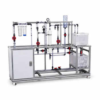
The key to unlocking filtration constants lies in a simple linear plot. Students can determine the filtration constants (K) and (q_e) using a laboratory-scale plate and frame filtration pilot plant by performing a constant‑pressure experiment. By recording the cumulative filtrate volume (V) over time (\theta), calculating the filtrate volume per unit filter area (q = V/A), and plotting (\theta/q) against (q), they obtain a straight line. The slope of this line equals (1/K) and its y‑intercept equals (2q_e/K), from which (K) and (q_e) are calculated directly.
The filtration constants (K) and (q_e) define the kinetics of cake filtration. With a plate‑and‑frame pilot plant, the only required data is a time series of filtrate volume under constant pressure. A (\theta/q) vs. (q) plot transforms this raw data into a straight line whose slope and intercept yield the constants—no complex curve fitting or proprietary software needed.
The Theory Behind the Filtration Constants
Before running the experiment, students must understand what they are measuring. The method is derived from the fundamental filtration equation for cake filtration, and the constants themselves carry physical meaning that connects to industrial design.
The Fundamental Filtration Equation
Under constant‑pressure conditions, the relationship between time (\theta) and the cumulative filtrate volume per unit area (q) is governed by the parabolic filtration equation:
[ \frac{\theta}{q} = \frac{1}{K} , q + \frac{2}{K} , q_e ]
This equation is the cornerstone of the entire exercise. It shows that if a student plots (\theta/q) on the y‑axis and (q) on the x‑axis, the data should fall on a straight line—provided the experiment genuinely obeys constant‑pressure cake filtration.
What Do (K) and (q_e) Represent?
Knowing the constants is only half the battle; understanding them is what makes the lab a learning experience.
(K) is the filtration constant (in m²/s). It encapsulates the overall permeability of the filtering system—specifically, it depends on the pressure drop, the specific cake resistance, the filtrate viscosity, and the concentration of solids in the slurry.
(q_e) is the equivalent filtrate volume per unit area (in m). It accounts for the resistance of the filter medium (the cloth itself). Conceptually, it’s the volume that would have to be filtered to build up a cake whose resistance equals that of the medium. A small (q_e) indicates a clean, low‑resistance medium; a large (q_e) points to a clogged or thick cloth.
By isolating (K) and (q_e), students can separate the resistance of the cake from that of the medium—the very same decomposition engineers use to scale up filtration processes.
Step-by-Step Experimental Procedure
The actual measurement on a plate‑and‑frame pilot plant is straightforward, but meticulous technique is essential to obtain linear, analysable data.
Setting Up the Constant‑Pressure Run
The experiment must be performed under constant pressure. On a pilot plant, this typically means adjusting a back‑pressure valve or a pump speed controller until the pressure drop across the filter (measured by a differential pressure transmitter) stabilises at a chosen value. Record the active filtration area (A) of the plate‑and‑frame pack—this is the total area of the cloth exposed to the slurry, and it is a fixed number provided in the plant manual.
Keep the slurry concentration and temperature constant throughout. A well‑mixed feed tank is essential; otherwise, settling changes the solids content and invalidates the assumption of constant resistance.
Collecting the Essential Data: Time and Filtrate Volume
Once pressure is steady, start the stopwatch and begin collecting filtrate in a graduated cylinder or, better, using an electronic balance with a data‑logging interface.
Record the cumulative filtrate volume (V) at regular time intervals (\theta). Initially, when the filtrate is fast, take readings every 10–20 seconds. As the cake builds and flow slows, extend the interval to 30–60 seconds. Continue until the flow rate becomes nearly constant or the cake is too thick to maintain pressure.
From Raw Data to Filtration Constants
For each time point, calculate (q = V/A), then compute the ratio (\theta/q). Plot (\theta/q) on the y‑axis versus (q) on the x‑axis.
The first few data points may deviate because the filtration has not yet reached stable cake‑formation conditions; it is standard practice to discard the initial transient data so that only the linear portion is analysed.
Perform a linear regression on the selected data to obtain the best‑fit line:
[ \text{slope} = \frac{1}{K} \qquad \text{intercept} = \frac{2q_e}{K} ]
From these, (K = 1/\text{slope}) and (q_e = (\text{intercept} \times K)/2). A high R² value confirms the validity of the constant‑pressure filtration model for the chosen slurry and medium.
Understanding the Trade-offs and Common Pitfalls
Even with the right equation, a plat-and-frame experiment can produce nonsensical constants if certain practical issues are not managed. Recognising these challenges turns a recipe into real engineering insight.
Maintaining Truly Constant Pressure
A plate‑and‑frame filter is a batch device, and as the cake grows, the overall resistance increases. If the pilot plant uses a centrifugal pump without a pressure‑control loop, the pressure can rise over time, deviating from the constant‑pressure assumption.
Students should monitor the pressure continuously and, if using a manual system, make small, frequent adjustments to the control valve to keep the pressure gauge rock‑steady. Modern pilot plants often have a PID controller—use it.
Neglecting the Initial Unstable Period
At the very start, there is no cake, and the medium resistance dominates. The parabolic filtration law does not hold in this phase.
Plotting all data often gives a curved (\theta/q) vs. (q) line. Resist the temptation to force a straight line through every point; omitting the first few unstable readings is not cheating—it is correct data handling.
Measurement Errors and Data Logging Benefits
Manual volume readings with a stopwatch and measuring cylinder introduce timing inaccuracies and parallax errors, which can obscure the linear trend.
Using a pilot plant equipped with digital sensors—an electronic balance for mass (converted to volume) and a data‑logging system—eliminates human lag and provides dense, accurate data. The denser the data, the more reliable the slope and intercept, especially when the filtration is rapid.
How to Apply This to Your Project
After successfully determining (K) and (q_e), students can use these constants to predict filtration behaviour at larger scales or for different operation times. The approach you prioritize depends on your learning objective.
- If your primary focus is experimental accuracy: Use digital data logging, maintain strict constant pressure via automatic control, and rigorously discard initial data points. Perform a linear regression with confidence interval analysis to quantify uncertainty.
- If your primary focus is understanding filtration theory: Vary the feed slurry concentration or pressure in separate runs. Plot the resulting (K) values against pressure to see how cake compressibility affects the constant, and use the values to calculate specific cake resistance and medium resistance.
- If your primary focus is a quick, repeatable demonstration: Keep the setup simple—clock and measuring cylinder—and emphasise the quality of the linear fit. Even a few well‑chosen data points on the stable portion can convincingly show the (\theta/q) vs. (q) relationship.
The plate‑and‑frame filtration experiment transforms an abstract transport‑phenomena equation into a tangible engineering tool, and the constants you extract are the direct link between a small‑scale lab run and a full‑sized industrial filter press.
Summary Table:
| Parameter/Step | Description / Action | Calculation Formula |
|---|---|---|
| Filtration Constant ($K$) | Measures overall system permeability and cake resistance | $K = 1 / \text{Slope}$ |
| Equivalent Volume ($q_e$) | Represents the resistance of the filter medium (cloth) | $q_e = (\text{Intercept} \times K) / 2$ |
| Linear Plotting | Plot $\theta/q$ (y-axis) against $q$ (x-axis) | $\text{Slope} = 1/K$; $\text{Intercept} = 2q_e/K$ |
Bring Practical Engineering to Life with LABPARK
Looking to upgrade your laboratory’s educational or research capabilities? LABPARK provides high-quality Educational and Vocational Unit Operations Pilot Plants in chemical engineering, bioprocess & biotech, and environmental & water treatment.
Whether you are a university, research institute, or enterprise, our pilot plants—including advanced plate and frame filtration systems—are engineered to deliver reliable, industry-scale data for your students and researchers.
Ready to elevate your lab? Contact LABPARK today to request a quote or consultation.
Related Products
- Constant Pressure Filtration Educational Unit Operations Pilot Plant
- Continuous Sieve-Plate Distillation Pilot Plant for Unit Operations Laboratory Education
- Plate Column Hydrodynamics Tray Demonstration Educational Pilot Plant
- Dual-Mode Rectification Pilot Plant for Practical Training Unit Operations
- Hot Filtration Educational Unit Operations Pilot Plant Laboratory System
People Also Ask
- How do educational unit operations pilot plants bridge theory and design? Bridge the Engineering Gap
- How do educational unit operations pilot plants address safety and waste management when scaling up?
- Why splitting a filtration batch doesn't always reduce cycle time? Pilot Plant Insights
- Why Demo Constant-Rate to Constant-Pressure Filtration on a Pilot Plant? Key Practical Insights
- How to select solid-liquid separation equipment for pilot plants? A Step-by-Step Guide