Researchers and instructors can estimate the characteristic diffusion time from the membrane thickness and the solute diffusivity using (t_D = L^2/D). Here, (L) should represent the relevant transport distance, usually the selective membrane layer, and (D) should be the solute’s effective diffusivity within that layer. The result provides the time scale for membrane penetration, sample scheduling, and interpretation of transient versus steady-state behavior.

The governing time scale is (t_D = L^2/D), so membrane thickness has a squared effect on response time. Use this value as an order-of-magnitude estimate, then account for external film resistance, module holdup, partitioning, and the specific criterion used to define “steady state.”

Calculating the Diffusion Time

Identify the Relevant Transport Thickness

Measure or obtain the thickness (L) of the membrane region that controls diffusion.

For an asymmetric membrane, this is generally the thin selective active layer, not the entire porous support. Using the total membrane thickness can substantially overestimate the intrinsic diffusion time when the support offers little resistance.

Obtain the Appropriate Diffusivity

Use the solute diffusion coefficient (D) inside the membrane material, with units such as (\mathrm{m^2/s}).

The appropriate value depends on membrane morphology:

In a dense, nonporous polymer, (D) describes molecular diffusion through the polymer.
In a porous membrane, transport may involve molecular diffusion, convection, or both.
For sufficiently small gas-filled pores, Knudsen diffusion may control transport.

When the membrane structure or operating conditions make a single diffusivity inadequate, use an effective diffusivity, (D_{\mathrm{eff}}), consistent with the selected transport model.

Apply the Characteristic-Time Equation

Calculate:

[ t_D = \frac{L^2}{D} ]

This is a diffusion time scale rather than an exact prediction of the time at which every point in a pilot module reaches steady state.

For example, if (L = 1.0 \times 10^{-6}\ \mathrm{m}) and (D = 1.0 \times 10^{-10}\ \mathrm{m^2/s}):

[ t_D = \frac{(1.0 \times 10^{-6})^2}{1.0 \times 10^{-10}} = 1.0 \times 10^{-2}\ \mathrm{s} ]

The intrinsic diffusion time through the selective layer is therefore approximately (0.01) seconds.

Interpreting Short-Time Penetration

Estimate the Penetration Depth

Before solute has penetrated the full membrane thickness, the approximate penetration depth is:

[ \delta(t) \approx (Dt)^{1/2} ]

This relationship is useful for interpreting startup data. If (\delta(t) \ll L), the solute has only entered part of the membrane and the measured flux may still reflect short-time transient behavior.

When (\delta(t)) becomes comparable to (L), the solute has had enough time to traverse the membrane thickness, and the membrane’s internal concentration profile begins approaching its long-time form.

Relate Penetration to Sampling

Sampling intervals should be selected in relation to (t_D), rather than chosen arbitrarily.

Early samples should be frequent enough to resolve the transient response. Later samples should be taken after the expected diffusion and hydrodynamic transients have diminished, particularly when the objective is to calculate steady-state flux or rejection.

Defining Steady State in a Pilot Plant

Use a Specified Stabilization Criterion

The phrase “time to steady state” requires a criterion. It may mean that the permeate concentration, retentate concentration, flux, or detector signal has changed by less than a specified percentage over a defined interval.

For some transient slab solutions, a practical estimate is written as:

[ t_{\mathrm{ss}} \approx 0.3\frac{L^2}{D} ]

This coefficient is model- and criterion-dependent. It should not replace (L^2/D) as the general characteristic scale unless it follows from the specific boundary conditions and steady-state definition being used.

Recognize the Square-Law Thickness Effect

Because time scales with (L^2), doubling the controlling membrane thickness increases the intrinsic diffusion time by a factor of four.

This relationship is especially important when comparing flat-sheet teaching modules, hollow fibers, and asymmetric commercial membranes with different selective-layer thicknesses.

Separate Membrane Response from Reservoir Decay

A membrane may reach a stable internal concentration profile while the feed reservoir continues to change concentration.

Researchers should therefore distinguish between:

Membrane equilibration, governed partly by (L^2/D).
Module or reservoir equilibration, governed by flow rates, holdup volumes, permeate removal, recirculation, and overall mass-transfer rates.

A stable instantaneous flux does not necessarily mean that the entire pilot-plant system has reached a global steady state.

Account for Resistances Outside the Membrane

Include External Film Resistance

The total mass-transfer resistance may be represented schematically as:

[ R_{\mathrm{overall}}

\frac{1}{k_1} + \frac{L}{DH} + \frac{1}{k_3} ]

where:

(k_1) is the feed-side mass-transfer coefficient,
(L/(DH)) represents the intrinsic membrane resistance,
(k_3) is the permeate-side mass-transfer coefficient,
(H) represents the relevant partition or solubility relationship.

The intrinsic diffusion time describes transport within the membrane. It does not, by itself, predict the response time of the complete module when the feed or permeate films dominate.

Evaluate Cross-Flow Conditions

Thin selective layers often have low intrinsic resistance, which makes external boundary layers more important.

Feed flow rate, channel geometry, mixing, viscosity, and cross-flow conditions affect (k_1) and (k_3). A pilot module may therefore respond more slowly than the membrane-only calculation suggests.

Include Module Holdup and Instrument Response

For continuous monitoring systems, the observed response can also include fluid-phase transport, dead volume, detector volume, and signal-processing delay.

The measured time constant may consequently be much longer than (L^2/D), even when membrane diffusion itself is rapid.

Choosing the Correct Transport Model

Neutral Solutes

For a neutral solute in a nonreactive membrane, Fickian diffusion and the (L^2/D) time scale are often an appropriate starting point.

The calculation remains an estimate, especially when concentration-dependent diffusivity or nonideal partitioning is significant.

Charged Solutes

For ions in charged membranes, diffusion may be coupled with electromigration and electrostatic partitioning.

A Nernst-Planck model, potentially combined with Donnan equilibrium, may be required. In such systems, the concentration response may not follow a simple linear diffusion model based only on the bulk concentration difference.

Suspensions and Slurries

When the feed contains particles, use an effective transport property when appropriate.

Particle obstruction, particle-phase partitioning, and suspension concentration can alter the apparent diffusivity. Substituting the diffusivity of the pure continuous liquid into (L^2/D) may therefore misrepresent the observed pilot-scale response.

Understanding the Trade-offs

The Formula Is Simple, but the Inputs Are Not

The calculation is only as reliable as the selected thickness and diffusivity.

A nominal membrane thickness may include a porous support that is not rate-limiting, while a tabulated diffusivity may apply to the solvent rather than to the actual membrane phase.

A Short Membrane Time Does Not Guarantee Fast Operation

A very thin selective layer can have a small intrinsic diffusion time, but the overall process may still be limited by external films, polarization, module residence time, or reservoir depletion.

The membrane estimate should therefore be compared with hydrodynamic and system-level time scales.

“Steady State” Can Be Misidentified

Using one calculated time and immediately declaring steady state is a common experimental error.

Steady state should be confirmed from measured flux or concentration data, with the selected variable remaining within a defined tolerance over a suitable observation period.

The 0.3 Factor Is Not Universal

The expression (0.3L^2/D) can be useful for a particular transient solution and stabilization criterion, but it is not a universal correction factor.

Boundary conditions, membrane geometry, initial conditions, and the chosen error tolerance determine the numerical multiplier.

Making the Right Choice for Your Goal

Use the diffusion estimate as the first step, then validate it against pilot-plant measurements.

If your primary focus is estimating intrinsic membrane response: Calculate (t_D=L^2/D) using the selective-layer thickness and the solute diffusivity within the membrane.
If your primary focus is selecting sampling intervals: Collect early samples on a time scale smaller than (t_D), then continue sampling until measured flux or concentration satisfies the defined stability criterion.
If your primary focus is obtaining steady-state separation data: Add sufficient time for external film, module holdup, and reservoir effects, and verify stabilization experimentally.
If your primary focus is comparing membrane designs: Examine the squared dependence on thickness and use morphology-appropriate effective diffusivities.
If your primary focus is modeling charged, porous, or slurry systems: Replace the simple Fickian estimate with the relevant coupled transport model and effective properties.

By treating (L^2/D) as a physically grounded time scale rather than an automatic steady-state guarantee, researchers and instructors can design more reliable membrane pilot-plant experiments.

Summary Table:

Key factor	Guidance
Characteristic time	Calculate `t_D = L^2/D`
Transport thickness	Use the selective membrane layer, not the full support
Diffusivity	Use the solute's effective diffusivity in the membrane
Penetration depth	Estimate with `delta(t) = (Dt)^(1/2)`
Thickness effect	Doubling thickness increases diffusion time fourfold
Steady-state estimate	`0.3L^2/D` may apply only to specific models and criteria
Additional delays	Consider film resistance, module holdup, reservoir decay, and instrument response
Complex systems	Use coupled transport models for charged, porous, or slurry systems

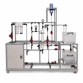
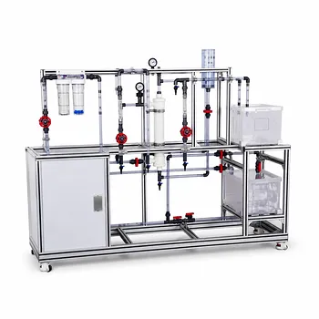
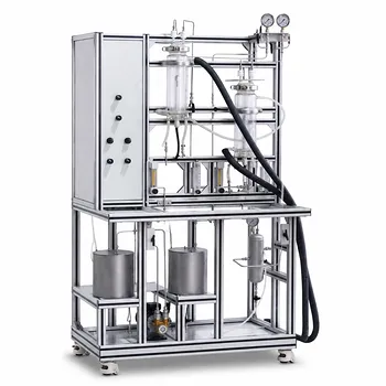
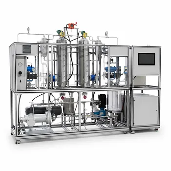
Planning membrane separation experiments or upgrading your teaching and research facilities? Contact LABPARK for Educational and Vocational Unit Operations Pilot Plants tailored to chemical engineering, bioprocess and biotech, and environmental and water treatment applications. LABPARK helps universities, research institutes, and enterprises select practical pilot-plant configurations, integrate reliable mass-transfer studies, and support accurate sampling, scale-up, and process evaluation.