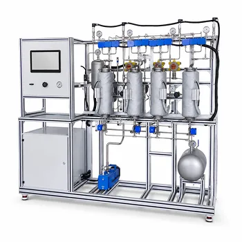
How Can Chemical Engineering Students Utilize The Kremser Equation To Calculate Theoretical Stages?

The Kremser equation gives you a direct, analytical route from lab measurements to theoretical stage count. By tracking just two gas-phase solute concentrations at the column inlet and outlet, you can compute the unabsorbed fraction, combine it with your known liquid-to-gas ratio and equilibrium data, and instantly solve for the number of ideal stages—no manual graphical stepping required. This turns a complex pilot-plant experiment into a precise, repeatable calculation that directly links operating conditions to separation performance.

The Kremser method is the preferred analytical shortcut for dilute gas absorption when the equilibrium line is linear. It eliminates the drawing errors of graphical techniques and lets you rigorously calculate theoretical stages from the easily measured unabsorbed solute fraction and the absorption factor. The real power comes from comparing this ideal stage count to your column’s actual physical stages, yielding a concrete plate or packing efficiency that grounds textbook theory in real equipment behavior.

Why the Kremser Equation Belongs in Your Gas Absorption Experiment

In a typical pilot-plant gas absorption run, you have a column with a known number of physical trays or a measured packed height. You also have control over the liquid and gas flow rates. What you don’t have is a direct readout of how many “perfect” stages your column actually achieves. The Kremser equation bridges that gap by calculating the number of theoretical stages (N) that would be required to achieve the measured separation, assuming ideal equilibrium on each stage.

The core relation—derived from mass balances and a constant equilibrium slope (m)—is:

[ N = \frac{\ln\left[ \left(1 - \frac{1}{A}\right) \frac{1}{\phi_A} + \frac{1}{A} \right]}{\ln A} ]

where:

(\phi_A) = unabsorbed solute fraction (a value you measure)
(A) = absorption factor (a value you control and calculate)

Once you have (N), the comparison with the actual number of trays or the equivalent theoretical plates from packing height becomes a straightforward stage efficiency calculation.

The Unabsorbed Fraction: Your One Critical Measurement

The entire experiment hinges on determining (\phi_A). This is simply the ratio of the solute leaving in the gas phase to the solute entering in the gas phase. For a dilute system with negligible gas-side volume change, you can work directly with mole fractions:

[ \phi_A = \frac{y_{\text{out}}}{y_{\text{in}}} ]

In practice, you sample the gas stream at the inlet (before contact) and at the outlet (after scrubbing) under steady-state conditions. Using a gas chromatograph or a calibrated detector, you obtain the solute mole fractions. A low (\phi_A) means excellent absorption; a value near 1 means poor removal.

The Absorption Factor: Where Operating Conditions Meet Thermodynamics

The absorption factor (A) is the ratio of the slope of the operating line to the slope of the equilibrium line:

[ A = \frac{L}{m,G} ]

(L) = molar liquid flow rate
(G) = molar gas flow rate
(m) = Henry’s law constant (or the linear equilibrium constant), taken from the linear portion of your solute’s equilibrium curve (y^* = m x).

You directly set (L) and (G) via rotameters or control valves. The value of (m) comes from phase equilibrium data at the column’s operating temperature and pressure. If (A > 1), the solvent can absorb the solute effectively; if (A < 1), the gas-phase solute is not sufficiently captured, and the required number of stages climbs rapidly.

Solving for N in One Step

Once (\phi_A) and (A) are known, plug them directly into the Kremser equation. In most educational experiments, you’ll use a spreadsheet or a simple calculator. The formula yields the minimum number of ideal stages needed to achieve the measured outlet concentration under the chosen L/G ratio.

Key insight: The equation assumes that each stage reaches equilibrium and that both the operating and equilibrium lines are straight. Because these conditions are rarely perfect in a real pilot plant, the computed (N) almost never matches the physical stage count—and that’s exactly what you want to investigate.

Turning Theoretical Stages into Real-World Efficiency

The whole point of the exercise is not just to calculate (N). It’s to ask: How well does my column perform relative to an ideal cascade?

You can compute the overall plate efficiency if you have a tray column:

[ E_o = \frac{N}{N_{\text{actual}}} \times 100% ]

Or, for a packed column, you divide the known packing height by (N) to get the Height Equivalent to a Theoretical Plate (HETP):

[ \text{HETP} = \frac{\text{Packed height}}{N} ]

Comparing these values across different gas and liquid flow rates lets you map how real fluid dynamics, channeling, and non-ideal mixing degrade performance.

Understanding the Trade-offs: When the Kremser Method Holds—and When It Falters

No analytical method is universal. Recognizing the boundaries of the Kremser equation is just as important as knowing how to use it.

The Dilute Assumption

The derivation assumes constant total molar flow rates of liquid and gas, which is valid only for dilute mixtures. If you are absorbing 10% or more of a soluble gas, the gas flow rate shrinks significantly from bottom to top, and the operating line is no longer straight. In such cases, a single absorption factor (A) is not constant, and the Kremser equation can lead to significant under- or over-estimation of stages.

Linear Equilibrium Requirement

The method works because the algebraic solution relies on a linear equilibrium relationship (y^* = m x + b). If your solute’s equilibrium curve bends noticeably over the concentration range you are operating in, the computed (N) becomes unreliable. For highly curved equilibria, you fall back to the graphical McCabe-Thiele step-off method or to more rigorous stage-to-stage calculations.

Constant Operating Line Slope

The L/G ratio must remain constant through the column. In a student pilot plant with well-mixed, steady flows, this is usually true. However, if temperature changes along the column (absorbers are sometimes exothermic), the liquid’s solvent capacity changes, altering the effective (m). This invalidates the single-value equilibrium constant. You must either maintain isothermal conditions or pick the mean (m) cautiously and acknowledge the error.

Ignoring Mass Transfer Resistances

The Kremser equation gives theoretical stages—each one assumes instantaneous equilibrium. Real trays or packing don’t achieve equilibrium. That’s why you compute efficiency. However, the analytical result alone cannot tell you about the rate limitations. If your goal is to understand mass transfer coefficients, the Kremser method is only a starting point; you’ll need to integrate HTU-NTU concepts or rate-based models as well.

Making the Right Choice for Your Experiment

Your approach depends on what you’re trying to learn and the nature of your absorption system.

If your primary focus is quantifying column efficiency under normal operating conditions: Use the Kremser equation with your measured (\phi_A) and carefully determined (A). The comparison of (N) to actual physical stages yields a clean efficiency metric that changes predictably with flow rates.
If you are working with a truly dilute, isothermal system and linear equilibrium data: The Kremser method is your most accurate and repeatable tool. It avoids the subjective errors of graphical stepping and allows quick sensitivity analyses on L/G and solute removal.
If your solute concentration is moderate or the equilibrium line is curved: Start with the Kremser result as an estimate, but then verify with a full McCabe-Thiele construction or a rigorous simulation. The analytical number gives you a baseline, while the graphical method captures curvature.
If you want to teach the link between thermodynamics and stage requirements: Have students first plot the equilibrium data and verify linearity, then apply the Kremser equation. This connects the chemical system’s properties directly to the stage demand, reinforcing the concept of the absorption factor.

By making the Kremser calculation the centerpiece of your gas absorption analysis, you move from “we ran a column” to “we quantified exactly how far our real column deviates from ideal behavior and why.” That’s the kind of concrete, data-driven understanding that turns a routine lab exercise into a genuine chemical engineering insight.

Summary Table:

Parameter	Symbol	Definition / Source	Role in Calculation
Unabsorbed Fraction	$\phi_A$	$y_{\text{out}} / y_{\text{in}}$ (measured)	Measures solute removal performance
Absorption Factor	$A$	$L / (m \cdot G)$ (flow rates & equilibrium)	Relates solvent capacity to gas flow
Theoretical Stages	$N$	Calculated via Kremser Equation	Benchmarks ideal column performance
Stage Efficiency	$E_o$ / HETP	$N / N_{\text{actual}}$ or $\text{Height} / N$	Quantifies real-world column deviation

Enhance Your Chemical Engineering Lab with LABPARK

Bring textbook thermodynamics to life with hands-on pilot plant experience. LABPARK designs and manufactures premium Educational and Vocational Unit Operations Pilot Plants in chemical engineering, bioprocess & biotech, and environmental & water treatment.

We help universities, research institutes, and enterprises bridge the gap between theory and practice with robust, safe, and highly visual training systems. Ready to elevate your laboratory capabilities?

👉 Contact LABPARK Today to Request a Quote