The definitive cause of flash simulation convergence failure is mathematical, not physical. When a flash algorithm refuses to converge, it’s almost always because the numerical solver has encountered a thermodynamic state it cannot resolve—either by landing on a physically meaningless solution or by oscillating around a phase boundary that doesn’t actually exist for the given conditions.
A flash calculation is fundamentally a root-finding exercise on a stability curve. Convergence failure is the algorithm's way of telling you it found a trivial root (K=1), a negative root, or no root at all—often because the specified temperature and pressure place the mixture entirely outside the two-phase envelope.
The Root of the Problem: Why Your Solver Gets Trapped
Before considering complex mixture effects, we must rule out basic algorithmic failure. These are the most common computational breakdowns that occur even for simple binary systems.
The Illusion of a Solution: The Trivial Root
The solver’s fundamental job is to minimize the Gibbs free energy of the system. A two-phase solution represents a global minimum. However, the algorithm can easily park itself on a trivial solution.
This happens when the vapor-liquid equilibrium ratios (K-values) all converge to 1.0. A K-value of 1.0 suggests the vapor and liquid compositions are identical, which is the definition of a single-phase mixture. The algorithm has successfully found a mathematical intersection but failed to find the physically correct, lower-energy two-phase split.
Choosing Sides: The Wrong Density Root
When solving a cubic equation of state, you are working with a polynomial in volume or compressibility factor (Z). For a two-phase system, this cubic equation yields three real roots.
The smallest root represents the liquid density. The largest root represents the vapor density. The middle root is physically meaningless—it represents an unstable state where pressure increases with volume. A simulation can easily fail if the algorithm inadvertently selects this unstable middle root or assigns the vapor root to the liquid phase during an iteration loop, sending the entire calculation into a non-physical spiral.
The Numerical Absurdity: Converging on a Negative Root
This is a fatal crash during iterative mathematics. As the solver adjusts density or compressibility guesses, the numerical method can overshoot. This drives the calculation into a mathematically valid but physically impossible realm where mass density or the compressibility factor becomes negative. This singular event instantly halts the simulation because subsequent flash calculations (like enthalpy departure) cannot process a negative mass.
The Phase Envelope Trap: When the Specs Don't Add Up
When the basic math is sound, the failure shifts to a thermodynamic mismatch. You may be ordering the algorithm to find two phases in a region where they fundamentally cannot coexist.
Operating Outside the Envelope
The most deceptive convergence failure occurs when there is no failure message, but an infinite loop of oscillations. You specify a temperature and pressure for the flash drum. If that point resides in the subcooled liquid region or the superheated vapor region, the algorithm's phase-splitting logic breaks down.
It calculates K-values that suggest the presence of a second phase, brings it in, then immediately determines the mixture is homogeneous and rejects it. This loop repeats, manifesting as a convergence failure because the true physical solution is a single-phase answer that the two-phase algorithm is not designed to accept.
The S-Curve Anomaly: Multiple Bubble Points
This is a critical issue in cryogenic or high-pressure systems with highly volatile, slightly soluble gases (like hydrogen in methane or nitrogen in heavy hydrocarbons). Under these conditions, the standard phase boundary becomes distorted.
At a constant pressure above the true critical pressure of the mixture, you don’t have a single bubble-point temperature. You can encounter an S-shaped bubble-point curve, yielding two or three valid bubble-point temperatures. A standard flash algorithm that uses a single initial temperature guess will lock onto the first bubble point it finds, even if that solution is a metastable liquid phase rather than the globally stable vapor phase. This misidentification causes the flash to fail or predict an erroneous, large vapor fraction.
The Instability Check Skipped
Equations of state are built to model stable phases. In the liquid region, the iterative solve can land on a mathematically correct but physically unstable solution. This is diagnosed by verifying the derivative of pressure with respect to volume (∂P/∂V). If ∂P/∂V is positive, the bulk modulus is negative, meaning the "liquid" is mechanically unstable and will spontaneously shatter into two phases. Algorithms that lack this check will hold onto this unstable state and eventually diverge.
Understanding the Trade-offs: Model Complexity vs. Stability
Not all equations of state are created equal when facing these convergence challenges. Your choice of model imposes hard constraints on the solver’s stability. Using a high-accuracy BWR-11 (Benedict-Webb-Rubin) equation for a simple pilot-plant simulation may actually be the root cause of your frustration. Its 11+ empirical constants create a highly non-linear surface that traps solvers in local minima, especially when initial estimates are poor. Simpler cubic models like Peng-Robinson or Soave-Redlich-Kwong are computationally far more rugged because their polynomial form is explicit and their root behavior is predictable, making them the workhorses for pilot plant design simulation. Furthermore, convergence failure is often a data problem. A model's default binary interaction parameters (kij) from a databank describe a generic mixture, not your specific chemical batch. If your pilot plant data shows a discrepancy, that is not a convergence failure but a prediction failure. Blindly adjusting kij to force convergence can create a model that represents your bench-top data but is thermodynamically inconsistent, leading to catastrophic scale-up errors. You must validate against a verified database like DIPPR or DECHEMA first.
Making the Right Choice for Your Pilot Plant Goal
Troubleshooting convergence requires matching your action to your root cause. Here is how to target your fix based on what you are trying to achieve:
- If your primary focus is eliminating a simple numerical crash: Implement a stability check that immediately rejects negative compressibility roots and validates ∂P/∂V < 0 before continuing the flash loop.
- If your primary focus is stabilizing a system with volatile gases like hydrogen: Do not use a standard flash. Implement a "multi-start" algorithm that uses different initial temperature guesses (e.g., 0.5x and 2x the feed temperature, plus the mixture's estimated critical temperature) to scan for and select the lowest Gibbs energy solution.
- If your primary focus is matching imperfect simulation data to pilot plant liquid levels: First, verify your specified feed state is inside the two-phase region, then cross-reference pure-component properties from a trusted physical property database before fine-tuning any binary interaction parameters.
You cannot brute-force a solution by tightening tolerances; you must help the algorithm find the physically meaningful root by eliminating the trivial and unstable ones.
Summary Table:
| Failure Cause | Primary Reason | Recommended Solution |
|---|---|---|
| Trivial Root | K-values converge to 1.0; no phase split found | Use better initial guesses & stability testing |
| Wrong/Negative Density Root | Solver selects unstable middle root or negative density | Implement constraint checks in algorithm |
| Operating Outside Envelope | Specified T & P lie in single-phase region | Verify feed state; allow single-phase solutions |
| S-Curve Anomaly | Multiple bubble points in cryogenic/volatile mixtures | Use multi-start temperature algorithms |
| Imperfect EOS Selection | Complex EOS (e.g., BWR-11) traps solver in local minima | Use rugged cubic models (PR or SRK) |
Verify Your Simulations with LABPARK Pilot Plants
Bridging the gap between computer models and real-world thermodynamic behavior is crucial for accurate scale-up. LABPARK provides state-of-the-art Educational and Vocational Unit Operations Pilot Plants in chemical engineering, bioprocess & biotech, and environmental & water treatment.
Designed specifically for universities, research institutes, and enterprises, our physical pilot systems help you validate simulation data, test phase equilibria, and eliminate modeling errors under real operating conditions.
Ready to enhance your research and training capabilities? Contact LABPARK today to find the perfect pilot plant solution for your facility!
Related Products
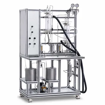
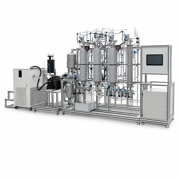
- Supercritical High-Gravity Flash Evaporation Educational Unit Operations Pilot Plant
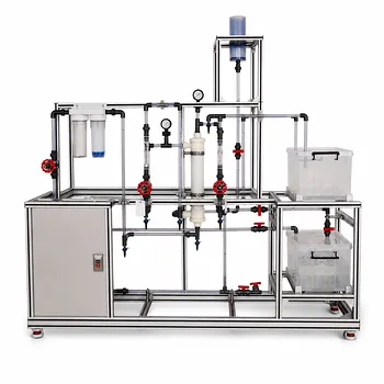
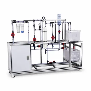
- Photocatalytic Membrane Separation and Degradation Unit Operations Pilot Plant
- Multi-Functional Membrane Separation Educational Pilot Plant for Unit Operations Lab
- Multi-Component Gas Pressure Swing Adsorption Pilot Plant for Unit Operations Education
- Hot Filtration Educational Unit Operations Pilot Plant Laboratory System
People Also Ask
- How is the heat transfer area calculated for an evaporation unit operations pilot plant during experimental design? Guide
- How to select educational evaporator pilot plants for thermal & scaling solutions? Complete Guide
- How to Connect Benchtop Evaporation to Pilot Plants in Chemical Engineering Education
- How are Dühring plots applied in evaporation pilot plants? Practical guide to boiling point prediction
- What is the practical significance of Kb in pilot plant evaporation? Master process design.