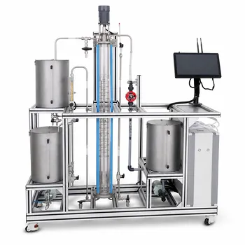
How To Apply Triangular Diagrams & Plait Points In Liquid-Liquid Extraction Pilot Plant Training

The triangular equilibrium diagram is your students' operational roadmap for the pilot plant, and the plait point is its most critical "do not cross" boundary.

It's used in two distinct phases. First, as a planning tool before startup: students plot their known feed and solvent compositions to find the mixing point on the diagram and use tie lines to predict the equilibrium compositions of the extract and raffinate phases. Second, as a real-time diagnostic tool during operation: they use the plait point to define the absolute maximum solute loading in the solvent (Y₂). In a water-acetic acid-benzene system, this limit is typically around 25% acetic acid to maintain a safe margin away from the plait point, preventing the two liquid phases from collapsing into one and stopping the extraction process entirely.

The core lesson is that a stable, operable extraction column depends entirely on staying within the two-phase envelope of the triangular diagram. The plait point is not just a theoretical concept; it’s the thermodynamic barrier that dictates your minimum solvent flow rate. Teaching students to use this diagram transforms column operation from a black-box activity into a predictable, controllable separation science.

Using the Diagram to Plan and Operate the Column

The diagram's primary function is to translate a theoretical separation problem into practical pilot plant settings. Students must learn that every point on the diagram represents a unique three-component mixture, and its location dictates whether separation is physically possible.

Mapping the Separation Before Startup

Before any fluid enters the column, the diagram serves as a predictive map. Students begin by plotting the feed (a mixture of water and acetic acid) and the pure solvent (benzene) on the right-angled triangle.

The line connecting these two points is the operating line. The mixing point (M) , which represents the overall composition of the combined feed and solvent stream entering the column, lies precisely on this line. Its exact location is calculated using a mass balance or the lever rule. This step visually demonstrates that extraction is simply a controlled mixing operation.

Verifying Phase Creation with Tie Lines

Once the mixing point is located, its significance is immediately clear. If point M lies within the two-phase envelope bounded by the binodal solubility curve, the mixture will split into two immiscible phases.

This is the pivotal moment where theory predicts reality. A tie line passing through point M connects the theoretical compositions of the exiting extract and raffinate phases. Students should then run the column to steady state, collect samples, and plot the actual exit compositions to see how closely they land on the ends of this theoretical tie line, graphically verifying the material balance.

The Plait Point as a Definitive Process Constraint

The plait point is where the compositional difference between the extract and raffinate phases shrinks to zero. Its location on the diagram defines the single most important operating limit for the pilot plant.

Why Approaching the Plait Point Destroys Separation

The plait point is the culmination of the two-phase envelope. As the solute (acetic acid) concentration increases, the compositions of the two liquid phases become more and more similar.

The visible consequence in the pilot plant’s glass column is dramatic. Students will observe the stable dispersion of droplets coalescing into a single, homogeneous phase as the solute concentration approaches the plait point. When this happens, the driving force for mass transfer—the difference from equilibrium—vanishes, and the column effectively becomes a simple mixer, not a separator.

Establishing the Safe Operating Limit

The educational value lies in teaching a quantitative safety strategy. The rule of thumb in a water-acetic acid-benzene system is to limit the acetic acid loading in the exiting solvent ($Y_2$) to roughly 25%.

This isn't an arbitrary number. It’s a practical margin of safety below the plait point. Students use this limit to calculate the minimum solvent flow rate needed. If the solvent flow is too low, the solute loading at the top of the column will exceed this threshold, taking the process dangerously close to the single-phase region. This directly links thermodynamic equilibrium data to a tangible, volumetric flow setting on the plant’s rotameter.

Teaching Verification, Performance, and Pitfalls

The final stage of instruction uses the diagram as a feedback loop to validate student findings and diagnose operational problems.

Constructing the Real-World Diagram from Plant Data

A powerful exercise is to have students build the diagram themselves. By running the column, deliberately taking compositions near the solubility limit, and titrating the phases, they can map out the experimental binodal curve and tie lines.

Plotting these self-derived curves against the literature data teaches a vital lesson in mass balance closure and analytical consistency. The visual scatter of their data points around the theoretical line is a direct, honest reflection of their experimental technique.

Understanding the Trade-offs

The Purity vs. Solvent Use Trade-off: A high solvent ratio easily keeps the process far from the plait point but yields a very dilute extract that requires costly downstream distillation. The diagram quantifies this trade-off, helping students find an economic optimum, not just a technically feasible one.
The Hazard of Misidentifying the Phase: A common student error is mislabeling which phase is the extract and which is the raffinate due to density differences. The triangular diagram serves as an independent check, as the compositions must align with the ends of the tie line.
The Assumption of Equilibrium: The diagram represents equilibrium, but a real column operates with finite kinetics. A large gap between the theoretical exit composition from the diagram and the actual sampled composition reveals inefficiencies due to low residence time, poor dispersion, or axial mixing. This gap is how students calculate the column's efficiency or its Height Equivalent to a Theoretical Stage (HETS).

Making the Right Choice for Your Pilot Plant Session

The depth to which you apply the diagram depends on your specific learning objectives. A single training module can't cover everything, so focus is key.

If your primary focus is demonstrating the fundamental principle of extraction: Focus entirely on the binodal curve. Use the diagram to show the single and two-phase regions, and then run the column at one condition deep inside the two-phase region so students can simply see the two immiscible phases in the glass column. The plait point here is just introduced as the boundary marker.
If your primary focus is teaching operational design and constraints: Center the entire session on a mass balance problem. Make students calculate the mixing point M, use the lever rule to predict flow rates, define the ~25% solvent loading limit, and then determine the resulting minimum solvent flow. The pilot plant run then validates whether their calculated settings actually work.
If your primary focus is performance analysis and troubleshooting: Have students generate their own experimental data to map the tie lines and calculate the number of theoretical stages. Use the plait point concept to then challenge them: "If your extract composition was too close to the plait point, what would you adjust on the column to fix it?" This forces them to bridge thermodynamics and mechanics.

Your ultimate goal is to ensure students leave the pilot plant not just knowing how to turn valves, but understanding the thermodynamic map that dictates every single action they take.

Summary Table:

Application Phase	Key Action	Practical Purpose & Constraints
Pre-Startup Planning	Plot feed, solvent, and mixing point (M) using the lever rule	Predicts phase separation and theoretical exit compositions
Real-Time Operation	Limit solute (acetic acid) loading to ~25%	Establishes a safety margin to prevent approaching the plait point
Performance Evaluation	Map experimental binodal curves and check tie lines	Validates mass balances and calculates column HETS/efficiency

Enhance your hands-on training curriculum with LABPARK. We design and supply high-quality Educational and Vocational Unit Operations Pilot Plants in chemical engineering, bioprocess & biotech, and environmental & water treatment for universities, research institutes, and enterprises. Equip your students with the tools to master complex thermodynamics and column operations in a safe, controlled environment—contact us today to find the perfect system for your lab!