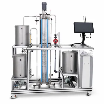
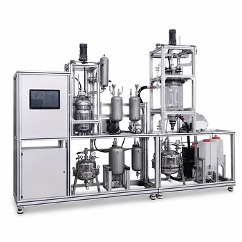
Transient solid-liquid diffusion is governed by Fick’s laws, conservation of mass, and the changing concentration difference between the solid and liquid phases. Inside the solid, solute moves by diffusion toward the surface; stirring transports that solute through the liquid and keeps the bulk liquid approximately uniform. Because the liquid volume is finite, its concentration rises as extraction proceeds, reducing the driving force until equilibrium or a specified recovery is reached.

Core takeaway: A pilot-scale extraction model must couple transient diffusion inside the solid with a dynamic liquid-phase mass balance. Internal diffusion, particle size, effective diffusivity, interfacial equilibrium, liquid volume, and agitation together determine the extraction rate and required batch time.

The Governing Physical Model

Fick’s First Law Determines the Local Flux

Fick’s first law relates solute flux to the concentration gradient:

[ \mathbf{N}A=-D{\mathrm{eff}}\nabla C_A ]

Here, (D_{\mathrm{eff}}) is the effective diffusivity of solute (A) through the solid matrix, and (C_A) is its concentration within the solid.

The negative sign indicates that solute moves from regions of high concentration toward regions of low concentration. In a porous particle, (D_{\mathrm{eff}}) reflects the effects of pore structure, porosity, tortuosity, saturation, temperature, and liquid viscosity.

Fick’s Second Law Describes Transient Depletion

For constant diffusivity and no reaction within the solid, the transient concentration field satisfies:

[ \frac{\partial C_A}{\partial t}

D_{\mathrm{eff}}\nabla^2 C_A ]

For a spherical particle, a common geometry in leaching models, this becomes:

[ \frac{\partial C_A}{\partial t}

D_{\mathrm{eff}} \left[ \frac{1}{r^2} \frac{\partial}{\partial r} \left( r^2\frac{\partial C_A}{\partial r} \right) \right] ]

The geometry matters because planar slabs, cylinders, and spheres have different diffusion path lengths and concentration profiles.

The Initial Condition Represents the Loaded Solid

The model begins with an initial solute distribution, often approximated as uniform:

[ C_A(r,0)=C_{A,0} ]

More complex solids may have a radial concentration profile caused by previous drying, impregnation, reaction, or precipitation. That initial condition can substantially affect the early extraction rate.

Symmetry Constrains the Particle Center

For a spherical particle, no net flux crosses the center:

[ \left. \frac{\partial C_A}{\partial r} \right|_{r=0}=0 ]

This condition prevents an artificial singularity at the center and reflects the physical symmetry of the particle.

How the Finite Liquid Volume Enters the Model

The Liquid Bulk Is Often Treated as Well Stirred

With vigorous agitation, the bulk liquid concentration can be approximated as spatially uniform:

[ C_L=C_L(t) ]

This assumption removes the need to solve a full liquid-phase concentration field. It does not remove mass transfer; it means that liquid-side concentration gradients are represented through an interfacial resistance or are assumed sufficiently small.

The Liquid Balance Couples Both Phases

The solute released from the solid accumulates in the finite liquid volume:

[ V_L\frac{dC_L}{dt}

\dot{m}_{A,\mathrm{solid\ to\ liquid}} ]

For (N_p) identical particles with surface area (A_p), this can be written as:

[ V_L\frac{dC_L}{dt}

N_p A_p N_A ]

where (N_A) is the outward solute flux at the particle surface.

The total solute balance provides an important consistency check:

[ M_{A,0}

M_A^{\mathrm{solid}}(t) + V_L C_L(t) ]

assuming no solute loss, degradation, or sampling removal.

Finite Volume Creates a Declining Driving Force

A commonly used interfacial condition is:

[ -D_{\mathrm{eff}} \left. \frac{\partial C_A}{\partial r} \right|_{r=R}

k_L\left(C_{A,i}-C_L\right) ]

where (C_{A,i}) is the liquid-equivalent interfacial concentration and (k_L) is the liquid-side mass-transfer coefficient.

If local equilibrium is represented by a partition relation,

[ C_{A,i}=K_{\mathrm{eq}}C_{A,s} ]

then the surface concentration in the solid and the liquid concentration are linked through (K_{\mathrm{eq}}). As (C_L) increases, the difference between the equilibrium liquid concentration and (C_L) decreases, so extraction slows.

The Key Dimensionless Principles

Fourier Number Measures Diffusion Progress

The dimensionless diffusion time is the Fourier number:

[ \mathrm{Fo}=\frac{D_{\mathrm{eff}}t}{R^2} ]

Here, (R) is the characteristic particle radius. Small values indicate that diffusion has penetrated only part of the solid, while larger values indicate more extensive depletion.

The characteristic diffusion time scales as:

[ t_D\sim \frac{R^2}{D_{\mathrm{eff}}} ]

This squared dependence makes particle size especially important in pilot-plant design. Halving the particle radius can reduce the characteristic internal diffusion time by approximately a factor of four, provided other limitations remain unchanged.

Biot Number Compares External and Internal Resistance

A mass-transfer Biot number compares liquid-side resistance with internal solid diffusion:

[ \mathrm{Bi}m=\frac{k_L R}{D{\mathrm{eff}}} ]

A large (\mathrm{Bi}_m) generally indicates that external resistance is relatively small compared with internal diffusion resistance. A small (\mathrm{Bi}_m) indicates that the liquid boundary layer may control or significantly influence the extraction rate.

The exact definition can vary with geometry and partitioning conventions, but the underlying question is the same: where does most of the concentration drop occur?

Similarity Solutions Explain Early-Time Behavior

For semi-infinite diffusion into or out of a solid, the similarity variable is:

[ \eta=\frac{x}{2\sqrt{D_{\mathrm{eff}}t}} ]

The diffusion equation can then produce error-function concentration profiles, such as:

[ \Theta(\eta)=\operatorname{erfc}(\eta) ]

These solutions show that the penetration depth grows with the square root of time:

[ \delta(t)\propto \sqrt{D_{\mathrm{eff}}t} ]

They are useful for understanding early extraction from large solids or thin surface layers, although finite-particle solutions are required once the diffusion front reaches the particle center.

Early Flux Often Decays as (t^{-1/2})

For an initially uniform semi-infinite solid exposed to a fixed surface concentration, the surface flux has the form:

[ N_A\propto \left(\frac{D_{\mathrm{eff}}}{\pi t}\right)^{1/2} \Delta C ]

The (t^{-1/2}) dependence describes the characteristic decline in transient diffusion flux. In a finite-volume extractor, the decline is usually stronger or otherwise modified because the liquid concentration changes and the available concentration difference decreases.

Applying the Model to Pilot Plants

Extraction Time Is a Coupled Design Variable

A pilot plant must provide enough contact time for the target fraction of solute to leave the solid. That time depends on (D_{\mathrm{eff}}), particle radius, temperature, solvent properties, liquid-to-solid ratio, equilibrium behavior, and agitation.

A simple estimate based only on (R^2/D_{\mathrm{eff}}) is useful for initial sizing, but it cannot predict the final recovery when liquid accumulation and equilibrium limitations are important.

Agitation Primarily Controls External Transport

Agitation reduces the liquid boundary layer surrounding particles and increases the liquid-side mass-transfer coefficient (k_L). It can also suspend particles, prevent settling, improve temperature uniformity, and reduce concentration gradients in the vessel.

Once external resistance becomes small, additional agitation produces diminishing improvements because internal solid diffusion has become the controlling resistance.

Particle Size Strongly Influences Throughput

Reducing particle size shortens the characteristic diffusion path and increases the available external surface area per unit mass. These changes usually accelerate extraction, but they may also increase energy consumption, create fines, complicate filtration, and cause handling or safety problems.

Pilot testing is therefore needed to identify the smallest practical particle size rather than assuming that maximum grinding is optimal.

Liquid Volume Controls the Driving Force

A larger solvent volume can keep the bulk liquid concentration lower for a given amount of extracted solute. This maintains a larger driving force and can increase the final recovery when equilibrium partitioning would otherwise limit extraction.

The trade-off is increased solvent use, larger downstream concentration duty, and potentially larger equipment volume. The appropriate liquid-to-solid ratio is therefore an optimization variable rather than a universal constant.

Pilot Data Connects Theory to Scale-Up

A useful pilot campaign measures bulk liquid concentration as a function of time while recording particle size, temperature, agitation speed, solvent volume, and solid loading. These data can be fitted to a transient diffusion model to estimate (D_{\mathrm{eff}}), (k_L), equilibrium parameters, or combinations of them.

Agitation speed alone is not a transferable scale-up criterion. Scale-up should preserve the controlling transport behavior, using relevant quantities such as mixing time, power input, suspension quality, Reynolds number, or experimentally correlated mass-transfer coefficients.

Understanding the Trade-offs

The Well-Stirred Assumption Has Limits

A liquid can appear vigorously mixed while still containing local concentration gradients near particles, vessel walls, or poorly suspended regions. If the liquid volume is large or the suspension is dense, a spatially uniform (C_L(t)) may be inaccurate.

Mixing-time measurements, tracer tests, or compartment and computational fluid-dynamics models can be used when bulk uniformity is uncertain.

Internal Diffusion May Not Be the Only Mechanism

The apparent extraction rate may include rapid surface washing, pore diffusion, swelling, particle breakage, dissolution, chemical reaction, adsorption, or desorption. Treating every deviation from ideal Fickian behavior as a change in diffusivity can produce misleading fitted parameters.

A reaction-diffusion model or a shrinking-particle model may be needed when the solid structure changes during extraction.

Effective Diffusivity Is Usually an Apparent Property

(D_{\mathrm{eff}}) is not necessarily the molecular diffusivity measured in a pure liquid. It often incorporates pore geometry, tortuosity, constriction, saturation, partitioning, and interactions with the solid matrix.

Its value may change with temperature, moisture content, solute concentration, or degree of depletion. A coefficient fitted at laboratory scale should therefore be validated under pilot conditions.

Equilibrium Can Limit Final Recovery

Increasing agitation cannot overcome an unfavorable equilibrium relationship. If the liquid approaches its equilibrium concentration, the extraction rate becomes small even when mixing is excellent.

Counter-current operation, solvent renewal, staged extraction, pH adjustment, or a selective chemical reaction can improve the overall driving force when these approaches are compatible with the product and process.

Multicomponent Systems Require Additional Care

For dilute single-solute extraction, a Fickian or pseudobinary model is often adequate. In concentrated or multicomponent systems, species interactions, competitive adsorption, nonideal thermodynamics, and coupled diffusion may require Stefan-Maxwell or other multicomponent transport descriptions.

The model should match the composition range and accuracy required for the pilot-plant decision.

How to Apply This to Your Project

A transient extraction model should be developed around measurable properties and validated against concentration-versus-time data. The following priorities help align the model with the engineering objective:

If your primary focus is extraction time: Estimate (R^2/D_{\mathrm{eff}}), measure particle-size distributions, and fit the full transient solid diffusion model to determine the batch time for the required recovery.
If your primary focus is agitation performance: Vary impeller speed or fluidization conditions while measuring extraction rate, suspension quality, and mixing time to separate liquid-side resistance from internal diffusion.
If your primary focus is solvent consumption: Use the finite-volume liquid balance and equilibrium relationship to select the liquid-to-solid ratio or number of extraction stages that achieves recovery with acceptable solvent use.
If your primary focus is pilot-to-production scale-up: Determine whether internal diffusion, external mass transfer, mixing, or equilibrium controls the process, then preserve the controlling dimensionless behavior and validate it at larger scale.
If your primary focus is model reliability: Check total mass conservation, measure temperature and viscosity, characterize porosity and particle size, and test whether (D_{\mathrm{eff}}) and (k_L) remain valid over the operating range.

The central engineering task is to identify the controlling resistance and design the pilot plant so that its measurements distinguish diffusion, mixing, and equilibrium effects.

Summary Table:

Principle	Role in Extraction Design
Fick's first law	Calculates solute flux from concentration gradients.
Fick's second law	Predicts transient solute depletion inside particles.
Finite liquid balance	Tracks rising bulk concentration and declining driving force.
Fourier number	Relates diffusion progress to time and particle size.
Mass-transfer Biot number	Compares external liquid resistance with internal diffusion.
Particle radius	Strongly affects extraction time, approximately proportional to R^2/D_eff.
Agitation	Increases liquid-side mass transfer, suspension, and temperature uniformity.
Equilibrium relationship	Determines the maximum achievable recovery.
Pilot data	Validates D_eff, k_L, equilibrium parameters, and scale-up assumptions.

Improve Your Extraction Pilot Plant

Need to determine extraction time, solvent volume, agitation requirements, or scale-up conditions? Contact LABPARK to discuss an Educational or Vocational Unit Operations Pilot Plant tailored to your project.

LABPARK helps universities, research institutes, and enterprises evaluate solid-liquid extraction using practical pilot-scale equipment for chemical engineering, bioprocess and biotechnology, and environmental and water-treatment applications. Our systems support controlled studies of particle size, temperature, liquid-to-solid ratio, agitation, mixing, mass transfer, and equilibrium so your team can identify the controlling resistance and generate reliable concentration-versus-time data.

Work with LABPARK to connect transient diffusion theory with measurable process performance, improve solvent and energy efficiency, validate scale-up parameters, and select operating conditions that achieve your target recovery.