The theoretical torque on a sphere rotating in creeping flow is (G=-8\pi\mu\omega R^3), where (G) is the hydrodynamic resistance torque, (\mu) is dynamic viscosity, (\omega) is angular velocity, and (R) is sphere radius. The negative sign indicates that the fluid torque opposes the sphere’s rotation; its magnitude is (8\pi\mu\omega R^3). In unit operations viscometry teaching equipment, this linear torque-speed relationship allows students to calculate viscosity directly from measured torque and rotational speed.

For a sphere rotating in an effectively unbounded fluid at very low Reynolds number, (\lvert G\rvert=8\pi\mu\omega R^3). Therefore, a torque measurement at known (R) and (\omega) gives (\mu=\lvert G\rvert/(8\pi R^3\omega)), provided creeping-flow and negligible-wall-effect assumptions are valid.

Why the Torque Is Linear in Angular Velocity

Creeping-flow conditions

The result applies when the Reynolds number is much less than one:

[ \mathrm{Re}\ll 1 ]

Under this condition, inertial effects are negligible compared with viscous effects. The fluid motion is therefore governed by the linear Stokes equations, making the resisting torque directly proportional to angular velocity.

Velocity field around the sphere

For a sphere rotating about an axis, the fluid velocity is purely azimuthal. In spherical coordinates, the velocity field is

[ v_\phi(r,\theta)=\frac{\omega R^3\sin\theta}{r^2} ]

where (r) is the distance from the sphere center and (\theta) is the polar angle measured from the rotation axis.

This field satisfies the no-slip condition at the sphere surface and decays away from the sphere.

Surface shear stress

The azimuthal shear stress at the sphere surface is obtained from

[ \tau_{r\phi}

\mu r\frac{\partial}{\partial r} \left(\frac{v_\phi}{r}\right) ]

Substituting the velocity profile and evaluating at (r=R) gives

[ \tau_{r\phi}(R,\theta)

-3\mu\omega\sin\theta ]

The stress is largest near the sphere’s equator, where (\sin\theta) is greatest, and vanishes at the rotational poles.

Deriving the Resistance Torque

Contribution from a surface element

A surface element on the sphere is

[ dA=R^2\sin\theta,d\theta,d\phi ]

The local moment arm about the axis of rotation is

[ R\sin\theta ]

Thus, the differential torque is the shear force on the surface element multiplied by this moment arm:

[ dG

\tau_{r\phi}(R,\theta) \left(R\sin\theta\right)dA ]

Integration over the sphere

Integrating over the full spherical surface gives

[ G

\int_0^{2\pi}\int_0^\pi \left(-3\mu\omega\sin\theta\right) \left(R\sin\theta\right) \left(R^2\sin\theta\right) ,d\theta,d\phi ]

Therefore,

[ G

-3\mu\omega R^3 \int_0^{2\pi}\int_0^\pi \sin^3\theta,d\theta,d\phi ]

Using

[ \int_0^{2\pi}d\phi=2\pi \qquad\text{and}\qquad \int_0^\pi\sin^3\theta,d\theta=\frac{4}{3} ]

produces

[ \boxed{G=-8\pi\mu\omega R^3} ]

The experimentally relevant resistance-torque magnitude is

[ \boxed{\lvert G\rvert=8\pi\mu\omega R^3} ]

How the Expression Is Used in Viscometry Teaching Equipment

Converting torque into viscosity

A teaching viscometer uses a motor to rotate the sphere at a known angular velocity and measures the torque required to maintain that rotation. Rearranging the theoretical expression gives

[ \boxed{\mu=\frac{\lvert G\rvert}{8\pi R^3\omega}} ]

Students can therefore determine dynamic viscosity from three quantities:

measured resistance torque, (G);
sphere radius, (R);
angular velocity, (\omega).

Demonstrating rotational viscometry

The equipment makes the physical meaning of viscosity measurable. A more viscous fluid produces greater resistance at the same rotational speed, while increasing the rotational speed produces a proportionally larger viscous torque.

The expected relationship is

[ \lvert G\rvert\propto\omega ]

A plot of measured torque against angular velocity should therefore be linear within the creeping-flow operating range. Its slope is

[ \frac{\lvert G\rvert}{\omega}=8\pi\mu R^3 ]

which can be used to calculate viscosity.

Connecting theory with unit operations

In a unit operations laboratory, the apparatus illustrates how transport properties are obtained from controlled mechanical measurements. Students connect the fluid-mechanics derivation to an operating procedure involving speed control, torque measurement, data collection, and viscosity calculation.

The experiment also shows why equipment geometry matters: the torque depends on the sphere radius through (R^3), so radius must be known accurately.

Reducing wall-interference corrections

The theoretical expression describes a sphere rotating in an effectively unbounded fluid. When the sphere is sufficiently separated from vessel walls, the ideal relationship can be applied without complex wall-interference corrections.

This makes the rotating-sphere arrangement useful for teaching the fundamental viscosity measurement principle in a relatively direct form.

Understanding the Trade-offs

The creeping-flow assumption is essential

The expression is valid for (\mathrm{Re}\ll1). At higher Reynolds numbers, inertial effects become significant and the torque may no longer vary linearly with angular velocity.

Consequently, increasing the speed indefinitely does not preserve the theoretical calibration.

Wall proximity can alter the measured torque

The derivation assumes that the surrounding fluid extends sufficiently far from the sphere. Nearby vessel walls restrict the flow and can increase the measured resistance torque.

If the apparatus does not provide adequate clearance, the ideal equation may underestimate the true viscosity unless a correction is applied.

Torque includes more than the ideal fluid contribution in practice

A real instrument may measure mechanical friction, bearing resistance, or sensor offsets in addition to the sphere’s hydrodynamic torque. These contributions should be identified through appropriate zero or baseline measurements where the apparatus permits.

The theoretical equation should be applied to the corrected hydrodynamic torque.

Geometry and operating conditions must remain controlled

The relationship assumes a sphere of known radius rotating steadily in a uniform, Newtonian fluid. Changes in sphere size, speed, temperature, or fluid condition can affect the interpretation of the measurement.

For teaching purposes, these variables should be recorded and held constant or treated explicitly during data analysis.

Applying the Relationship in the Laboratory

The practical calculation follows directly from the theoretical result:

[ \mu=\frac{\lvert G\rvert}{8\pi R^3\omega} ]

If your primary focus is determining viscosity: Measure the steady resistance torque at a known angular velocity and calculate (\mu) using (\lvert G\rvert/(8\pi R^3\omega)).
If your primary focus is validating the theory: Measure torque over several low-speed operating points and test whether the torque-versus-speed relationship is linear.
If your primary focus is teaching experimental limitations: Compare the ideal prediction with measurements while considering Reynolds number, wall proximity, mechanical drag, and temperature.
If your primary focus is equipment calibration: Use a fluid of known viscosity to verify the torque response and identify any baseline torque or systematic deviation.

The rotating-sphere experiment turns the Stokes-flow torque law into a direct, teachable method for measuring viscosity and evaluating the assumptions behind unit operations instrumentation.

Summary Table:

Key aspect	Summary
Torque expression	(G=-8\pi\mu\omega R^3)
Torque magnitude	(
Viscosity calculation	(\mu=
Validity	Creeping flow with (\mathrm{Re}\ll1)
Expected trend	Resistance torque increases linearly with angular velocity
Main variables	Torque, sphere radius, angular velocity, temperature, and fluid condition
Practical considerations	Account for wall effects, mechanical friction, sensor offsets, and calibration

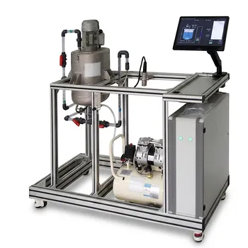
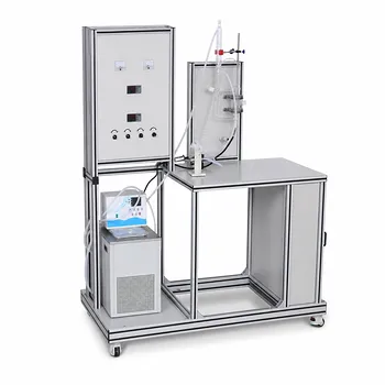
Bring fluid-mechanics theory into practical laboratory training with LABPARK Educational and Vocational Unit Operations Pilot Plants. Our viscometry teaching equipment helps universities, research institutes, and enterprises demonstrate rotational torque, viscosity measurement, creeping-flow behavior, calibration, and experimental limitations. Explore LABPARK's chemical engineering, bioprocess and biotech, and environmental and water treatment pilot plants, then contact LABPARK to discuss your teaching, research, or process-training requirements and identify the right equipment configuration.