Preparing a precise pH buffer is a foundational skill for any chemical engineering laboratory instructor. The explicit calculation for a pH 9.20 ammonia-ammonium chloride buffer involves determining a critical base-to-salt ratio from the ionization constant Kb and converting that into the masses and volumes required. For 500 cm³ of buffer with a final ammonia concentration of 1.0 mol·dm⁻³, you need 29 g of solid ammonium chloride and 33 cm³ of concentrated ammonia (15 mol·dm⁻³).
A buffer’s reliability isn’t just in the numbers—it’s in the discipline behind them. The core calculation uses the relationship [NH₃]/[NH₄⁺] = [OH⁻]/Kb to arrive at a ratio of 0.89. When you dissolve 29 g NH₄Cl in the ammonia and dilute to volume, you’ve satisfied the stoichiometry that theory demands. Yet, as every seasoned instructor knows, mastering the why behind each step is what transforms a simple preparation into a robust, reproducible experiment.
The Core Calculation: From pH to Mass and Volume
Why This Buffer Matters in Chemical Engineering Education
Ammonia-ammonium chloride buffers are ubiquitous in unit operations—absorption columns, liquid-liquid extraction, and reactive separation experiments often require a stable alkaline pH near 9.20.
An instructor who can derive the recipe from first principles not only guarantees experimental consistency but also models the rigorous thinking expected of future engineers.
Mapping pH to the Required Hydroxide Concentration
A pH of 9.20 translates directly into a pOH of 4.80 (14.00 – 9.20).
This gives a hydroxide ion concentration [OH⁻] = 1.6 × 10⁻⁵ mol·dm⁻³.
We now have the single ionic anchor needed to engage the ammonia ionization equilibrium.
Applying the Base Ionization Constant (Kb)
For the weak base ammonia, the equilibrium is NH₃ + H₂O ⇌ NH₄⁺ + OH⁻, with Kb = 1.8 × 10⁻⁵.
The defining relationship is Kb = [NH₄⁺][OH⁻] / [NH₃], which rearranges to the essential ratio:
[NH₃] / [NH₄⁺] = [OH⁻] / Kb = (1.6 × 10⁻⁵) / (1.8 × 10⁻⁵) = 0.89
This 0.89 ratio is the heart of the preparation—it fixes the relative amounts of the weak base and its conjugate acid that will resist pH change at 9.20.
The Step-by-Step Breakdown
Determining the Target Concentration Ratio
Using the ratio above, the buffer must contain ammonia and ammonium ions in a 0.89∶1 relationship.
You can think of it as: for every 1.0 mol of NH₄⁺, you need 0.89 mol of NH₃.
Converting the Ratio into Concrete Concentrations
The instructor’s chosen final ammonia concentration is 1.0 mol·dm⁻³.
To satisfy the 0.89 ratio, the ammonium ion concentration must be higher: [NH₄⁺] = 1.0 mol·dm⁻³ / 0.89 ≈ 1.1 mol·dm⁻³.
This 1.1 M NH₄⁺ is the target we will now turn into a mass of solid salt.
Calculating the Mass of Solid Ammonium Chloride
The source of NH₄⁺ is solid NH₄Cl (molar mass 53.5 g·mol⁻¹).
For a final volume of 0.50 dm³ (500 cm³):
Mass NH₄Cl = 0.50 dm³ × 1.1 mol·dm⁻³ × 53.5 g·mol⁻¹ ≈ 29 g
Weighing out 29 g of dry ammonium chloride ensures the conjugate acid concentration is correct.
Finding the Volume of Concentrated Ammonia Stock
Concentrated ammonia solution is typically 15 mol·dm⁻³.
To deliver 1.0 mol of NH₃ per litre in the final 0.50 dm³, the required volume is:
V(NH₃) = (1.0 mol·dm⁻³ × 500 cm³) / 15 mol·dm⁻³ ≈ 33 cm³
This small volume of intensely concentrated base is diluted to give the final 1.0 M ammonia.
The Preparation Procedure in Practice
Dissolve the 29 g of NH₄Cl in a small amount of distilled water in a 500 cm³ volumetric flask.
Add the 33 cm³ of concentrated ammonia, then carefully top up with water to the graduation mark and mix thoroughly.
This method guarantees the concentrations you mathematically designed.
Beyond the Calculation: Ensuring Accuracy in the Lab
The Hidden Influence of Temperature
The Kb value of 1.8 × 10⁻⁵ is strictly valid at 25°C.
If the laboratory temperature differs—say, on a warm afternoon—the equilibrium shifts, and the actual buffer pH may drift by several hundredths of a unit.
Always measure the final buffer at the intended experimental temperature and note the value for students.
Concentration vs. Activity: When Theory Meets Reality
The Henderson-Hasselbalch relationship uses concentrations, but real solutions behave according to activities.
In a buffer with an ionic strength of ~1 M, activity coefficients can alter the effective [NH₄⁺]/[NH₃] ratio, causing a small discrepancy between calculated and measured pH.
For demonstration purposes this is usually acceptable, but a precision experiment demands post-preparation pH verification and adjustment.
Stock Reagent Quality Over Time
Ammonia solutions lose strength because the gas is volatile; a stock labeled 15 M may be weaker.
Similarly, solid NH₄Cl can absorb moisture, altering the weighed mass’s actual salt content.
Standardizing the ammonia concentration via titration or using freshly opened, desiccator-stored NH₄Cl are habits that protect decades of pilot-plant results.
Understanding the Trade-offs and Common Pitfalls
The Simplicity-Accuracy Trade-off
The calculated recipe is fast and theoretically sound, giving a pH very close to 9.20.
However, a strictly “blind” preparation might yield pH 9.15 or 9.25 if non-idealities are present.
Instructors must weigh whether that ~0.1-unit uncertainty is acceptable for a teaching lab versus a research-grade investigation where the buffer must be dialed in with a calibrated pH meter.
Ionic Strength Effects on Unit Operation Data
In a packed-tower absorption experiment, the buffer’s ionic strength influences gas solubility (salting-out effects).
If the calculation ignores activity corrections, the actual [OH⁻] and gas-liquid equilibrium constants may shift, leading students to misinterpret mass transfer coefficients.
Acknowledging this pitfall—and possibly pre-adjusting the buffer while measuring conductivity—turns a source of error into a valuable systems-thinking lesson.
Common Volumetric and Weighing Missteps
Pouring 33 cm³ of ammonia from a beaker without allowing it to drain completely introduces volume errors.
Dissolving NH₄Cl in insufficient water and topping up before complete dissolution leads to a final volume that is off.
Use a clean volumetric flask, rinse all transfer vessels, and allow the solution to come to thermal equilibrium before the final dilution—small disciplines that compound into large reproducibility gains.
The Danger of Assumed Stock Concentrations
Taking “15 M” ammonia at face value can undermine the whole buffer calculation.
A 10% drop in stock concentration means your final NH₃ concentration is 0.9 M instead of 1.0 M, altering the ratio and the pH.
For critical experiments, the instructor should verify stock concentration by density measurement or acid-base titration.
Making the Right Choice for Your Goal
- If your primary focus is teaching buffer fundamentals: Use the exact calculated amounts (29 g NH₄Cl, 33 cm³ ammonia). Then, when the measured pH deviates slightly, unpack the science of activity, temperature, and reagent purity with your students—it becomes a rich, memorable lesson.
- If your primary focus is high-reproducibility research-grade rigs: Prepare the buffer by the calculation, then titrate the final solution to pH 9.20 using a freshly calibrated meter. Document any minor additions so future researchers can replicate your exact method.
- If your primary focus is scaling up for a pilot unit operation: Multiply the recipe linearly, but verify the final pH after each scale-up step. Pre-dissolve the NH₄Cl completely before adding ammonia, and consider preparing a concentrated stock if many batches are needed—just remember to re-check the pH after dilution.
When the cold logic of the Henderson-Hasselbalch equation is matched with artful laboratory technique, the result is a buffer that doesn’t just hit a number—it empowers an entire unit operations experiment with trustworthiness.
Summary Table:
| Parameter / Component | Value / Specification | Role in Buffer |
|---|---|---|
| Target pH | 9.20 (pOH 4.80) | Final solution acidity |
| Base-to-Salt Ratio ($[NH_3]/[NH_4^+]$) | 0.89 | Determines buffer capacity |
| Ammonium Chloride ($NH_4Cl$) | 29 g (1.1 mol/dm³) | Conjugate acid source |
| Concentrated Ammonia ($NH_3$) | 33 cm³ (15 mol/dm³) | Weak base source |
| Final Volume | 500 cm³ (diluted with distilled water) | Total solution volume |
Bring Industrial Precision to Your Engineering Labs
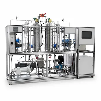
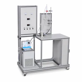
Translating theoretical calculations into successful physical experiments requires robust, reliable equipment. LABPARK provides state-of-the-art Educational and Vocational Unit Operations Pilot Plants in chemical engineering, bioprocess & biotech, and environmental & water treatment.
We help universities, research institutes, and enterprises bridge the gap between classroom theory and real-world process engineering.
Contact LABPARK today to discover how our pilot plants can enhance your training and research capabilities.
Related Products
- Alkaline Membrane Water Electrolysis Educational Pilot Plant Unit Operations Training System
- Ion Exchange Water Purification Educational Pilot Plant for Engineering Unit Operations
- Electrolyte Distillation Purification and Formulation Educational Pilot Plant
- Potassium Salt Thermal Dissolution and Crystallization Separation Educational Unit Operations Pilot Plant
- Carbon Dioxide PVT Curve Determination Educational Unit Operations Pilot Plant
People Also Ask
- How do chemical engineering pilot plants demonstrate electrolysis? Bridge Theory & Industrial Scale
- How do composite membranes affect NaOH production? Key factors for high current efficiency.
- Gap-Electrode vs. Zero-Gap Membrane: Key Design Choices for Water Electrolysis Pilot Plants
- What are the core parameters of water electrolysis efficiency? Master them with pilot plants.
- How do alkaline and PEM electrolysis technologies differ in pilot plant operations?