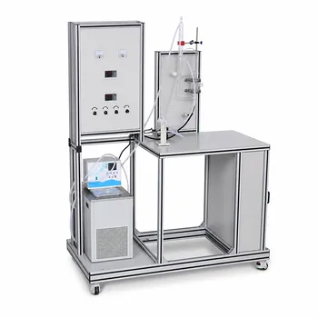
How Should Pressure Variations Be Accounted For In Liquid And Vapor Enthalpies? Pilot Plant Guide

For liquid streams in pilot plants, pressure variations have a negligible impact on enthalpy at constant temperature. You can treat liquid enthalpy as if it were a saturated liquid at the same temperature—no pressure correction is needed. For vapor streams, the picture is different: increasing pressure at a constant temperature drives the enthalpy downward, causing it to converge toward the saturated vapor dew point line. This simple behavior lets you build reliable heat load models by interpolating between two known pressure‑reference states (like 1 atm and 100 atm), all the way up to the supercritical single‑phase zone.

Core takeaway
Liquids behave like incompressible fluids—their enthalpy barely moves with pressure, so saturated‑liquid data is sufficient. Vapors, in contrast, compress; their enthalpy slides toward the saturation curve as pressure rises. By exploiting this predictable convergence, you can use a straightforward pressure‑interpolation method to obtain accurate vapor enthalpies without complex equations of state, dramatically simplifying pilot‑plant thermal calculations.

Why Pressure Reshapes Vapor Enthalpy

Pilot‑plant operations often swing over wide pressure ranges—from atmospheric distillation to high‑pressure gas‑liquid absorption. Understanding why pressure changes the enthalpy of a vapor, and not a liquid, is the key to choosing the right approximation.

The Convergence Toward the Dew Point Line

Picture the pressure‑enthalpy diagram for a pure fluid. At a constant temperature, as you increase the pressure on a superheated vapor, its enthalpy value moves closer to the saturated vapor line (the dew point).
Eventually, at the saturation pressure for that temperature, the vapor is about to condense and its enthalpy equals the saturated vapor enthalpy. This convergence happens because high pressure compresses the gas, reducing the average distance between molecules and altering the internal energy and the flow work contribution ((Pv)).

Entropy and Molecular Freedom in Compressed Gases

The effect has a thermodynamic root in entropy. When you pressurize a gas—say, from 101 kPa to 606 kPa—the volume shrinks, restricting molecular motion and the number of accessible microstates.
Lower entropy at a fixed temperature means less “dispersed” energy, which shows up in the enthalpy value. The same mechanism explains why gaseous reaction enthalpy data must be corrected for pressure; ignoring it can skew heat duty forecasts and equipment sizing.

Why Liquid Enthalpy Ignores Pressure

Liquids are far denser and far less compressible than gases. Squeezing a liquid with extra pressure does almost no work on the fluid, and the molecular packing barely changes.
Consequently, the enthalpy of a liquid at a given temperature stays essentially constant whether you are at 1 bar or 100 bar. The tiny variations sit well within the measurement uncertainty of most pilot‑plant instrumentation.

Using Saturated Liquid Data as a Reliable Proxy

Because pressure doesn’t move the needle, you can pull liquid enthalpy straight from a saturated‑liquid table at the stream temperature.
No pressure‑interpolation step is required. This shortcut is standard practice in industrial process simulators and—when backed by solid reference data—gives excellent accuracy for heat‑balance calculations on reboilers, preheaters, and liquid‑phase reactors.

A Practical Interpolation Method for Vapor Enthalpy

For vapor, the key insight is that the phase envelope provides a natural bounding reference.
If you know the saturated vapor enthalpy at the dew point and the ideal‑gas enthalpy (or a low‑pressure reference like 1 atm) at the same temperature, you can interpolate linearly—or with a slightly refined correlation—to find the enthalpy at any intermediate pressure, provided you stay below the supercritical limit.

Step‑by‑Step Interpolation Logic

Pick a temperature for your vapor stream.
Obtain two reference enthalpies at that temperature: one at a low pressure (e.g., 1 atm, approaching ideal‑gas behavior) and one at a high pressure (e.g., the saturation pressure for the dew point, or a fixed high value like 100 atm).
Assume enthalpy varies smoothly with pressure between these two points. A linear interpolation often suffices; where higher accuracy is needed, use a logarithmic or quadratic weighting based on tabulated data from a property database such as Maxwell.
Read the interpolated enthalpy for your operating pressure.

This approach dramatically cuts the complexity of pilot‑plant energy balances while preserving engineering accuracy.

When to Refine the Method Near the Critical Point

As you approach the supercritical single‑phase zone, the curvature of the pressure‑enthalpy surface becomes more pronounced.
In that region, a linear interpolation between 1 atm and 100 atm may drift several percent. The remedy is to use a third reference point—such as data at 50 atm—or to switch to a short‑cut equation of state that still avoids full‑scale iterative calculations.

Understanding the Trade‑offs and Limitations

Every simplification hides a trade‑off. The pressure‑invariant liquid enthalpy assumption works spectacularly for most applications, but it can introduce a small bias in ultra‑high‑pressure polymerisation or deep‑well pilot loops.
For vapor, the interpolation method hinges on the quality of your reference data. If your source database contains inaccurate dew‑point enthalpies, the entire heat‑load calculation will drift. Additionally, this method decouples pressure from temperature effects; if your process experiences simultaneous temperature and pressure swings, you must first compensate for temperature before applying the pressure‑interpolation rule.
For supercritical streams, the concept of a “dew point” disappears. Here, a single‑phase fluid model is necessary, and the simple two‑point interpolation should be replaced with a direct equation of state or a database lookup covering the precise temperature‑pressure pair.

Making the Right Choice for Your Pilot‑Plant Goal

The practical approach you adopt should match the dominant energy balance driver in your unit operation.
Choose your strategy based on what drives your heat‑load accuracy the most.

If your primary focus is liquid‑loop heat duties (preheaters, coolers, reboilers): Use saturated liquid enthalpy values at the stream temperature. Pressure adjustment is unnecessary and can be safely omitted from the calculation spreadsheet.
If your primary focus is vapor‑phase energy balances (overhead condensers, distillation columns, flash vessels): Apply the pressure‑interpolation method using at least two known enthalpy references at your process temperature. This captures the non‑ideal gas behaviour without resorting to heavy‑duty thermodynamics software.
If your primary focus is reactions or separations near the critical point: Supplement the interpolation with a third data point or a dedicated property correlation. Validate the results against reliable thermodynamic databases to avoid compounding errors in scale‑up designs.
If your primary focus is teaching or research demonstrations: Start with the simplified methods to illustrate the insensitivity of liquid enthalpy and the convergence of vapor enthalpy. Then let students compare the simplified results with rigorous simulations, turning the approximation into a powerful learning moment.

When you match the enthalpy calculation strategy to the phase and pressure regime of your pilot plant, you strike the right balance—speed, clarity, and the engineering accuracy needed to design, operate, and scale up with confidence.

Summary Table:

Phase	Pressure Sensitivity	Calculation Approach	Key Recommendation
Liquid	Negligible	Saturated liquid proxy at stream temperature	Ignore pressure corrections for standard loops
Vapor	Significant (high pressure lowers enthalpy)	Interpolation between low and high reference states	Interpolate between 1 atm and dew point values
Supercritical	Highly sensitive / non-linear	Direct Equation of State (EOS) or database lookup	Avoid simple interpolation near critical points

Optimize Your Unit Operations with LABPARK

Designing accurate thermal models is crucial for successful scale-up. LABPARK provides state-of-the-art Educational and Vocational Unit Operations Pilot Plants in chemical engineering, bioprocess & biotech, and environmental & water treatment. Designed specifically for universities, research institutes, and enterprises, our robust systems bridge the gap between thermodynamic theory and hands-on industrial practice.

Ready to elevate your lab's training and research capabilities? Contact us today to find the perfect pilot plant solution for your institution!