How Is The Rachford-Rice Equation Applied To Determine Vapor-Liquid Fraction? Optimize Pilot Plant Flash Experiments.

Simply put, the Rachford-Rice equation is solved iteratively—typically with the Newton-Raphson method—to find the molar vapor fraction (e). You feed it your known feed composition (z_i) and phase equilibrium constants (K_i), then refine an initial guess until the function (G(e)) equals zero. This calculated (e) instantly gives you the vapor and liquid flow rates, and from there you can back-calculate the equilibrium compositions of both phases to validate your pilot plant’s experimental mass balances.

In an isothermal flash experiment, the Rachford-Rice equation transforms abstract thermodynamic data into a hard number: the fraction of your feed that vaporizes. That single result is the bridge between the theoretical vapor-liquid equilibrium model you trust and the physical separation you observe, making it the gatekeeper for verifying whether your pilot plant behaves as predicted.

Why the Flash Drum Matters in Your Pilot Plant

Before running a distillation column, most educational and research pilot plants place a flash drum right after the feed pump. This single-stage separation vessel does the rough work—stripping out the lightest components—before the mixture hits the main column.

Reducing the Load on Downstream Equipment

By doing a preliminary cut, the flash drum lowers the thermal duty on the distillation column. That means smaller reboiler and condenser requirements, and a simpler overall energy balance to track during academic experiments.

Creating a Living Laboratory for VLE Models

An isothermal flash is the purest expression of vapor-liquid equilibrium you can physically build. The drum maintains a constant temperature, so every measured output becomes a direct test of the equilibrium constants ((K_i)) you selected from a thermodynamic model like Raoult’s Law, Wilson, or UNIQUAC. If the model’s predicted split doesn’t match what you collect in the product tanks, you’ve just found a gap in your understanding.

Applying the Rachford-Rice Equation, Step by Step

To actually use the equation in your pilot plant, you don’t just “plug and chug.” The process is a deliberate, four-step loop that connects your pressure gauges and sample ports to the core math.

Step 1: Assemble the Input Data

Your feed composition (z_i) comes directly from the known recipe or a compositional analysis. The temperature and pressure inside the flash drum—read off your pilot plant’s transmitters—define the state for which you’ll obtain the (K_i) values. If your temperature measurement drifts, your entire flash calculation shifts.

Step 2: Define the Objective Function

The Rachford-Rice equation is written as a root-finding problem:

(G(e) = \sum \frac{z_i(K_i - 1)}{(K_i - 1)e + 1} = 0)

Here, (e) is the molar vapor fraction ((V/F)). This function is monotonic for valid (e) between 0 and 1, which is why Newton-Raphson works reliably—provided your (K_i) values and (z_i) are physically consistent.

Step 3: Iterate with Newton-Raphson

Starting from an initial guess (typically (e = 0.5)), you update (e) using:

(e_{\text{new}} = e_{\text{old}} - \frac{G(e)}{G'(e)})

Where (G'(e)) is the derivative. In a pilot plant control room, this loop runs in a spreadsheet or a small script, and convergence usually takes fewer than 10 iterations. Each iteration brings the calculated vapor split closer to the one nature imposes inside the vessel.

Step 4: Recover Phase Flow Rates and Compositions

Once (e) converges, the liquid fraction is simply (L/F = 1 - e). With measured feed flow rate (F), you immediately know (V) and (L). The phase compositions come from material balance:

Vapor: (y_i = \frac{z_i K_i}{(K_i - 1)e + 1})
Liquid: (x_i = \frac{z_i}{(K_i - 1)e + 1})

These predicted numbers are what you compare against the actual samples pulled from the vapor outlet and liquid bottom of the pilot plant.

Connecting the Calculation to Experimental Mass Balances

The power of the Rachford-Rice equation in a pilot plant isn’t theoretical—it’s forensic. You can now close both the overall and component mass balances.

Spotting Measurement or Model Errors

If your total collected vapor and liquid masses don’t match the split predicted by (e), you have a gross error: perhaps a leaking valve, a miscalibrated flow meter, or a feed that’s not at steady state. If the overall mass balance closes but a single component’s measured (y_i) is off, you’ve likely chosen the wrong (K_i) model for that chemical system. The equation thus serves as both a design tool and a diagnostic instrument.

Verifying the Isothermal Assumption

In a perfect isothermal flash, the temperature is uniform and set by the heating jacket. The Rachford-Rice solution naturally rests on this assumption. A significant mismatch between the calculated (e) and the observed split can also indicate that your vessel isn’t truly isothermal—perhaps heat loss is condensing vapor on the walls, reducing the effective vapor fraction.

Understanding the Trade-offs

No tool comes without sharp edges. The Rachford-Rice equation’s clean mathematics rely on several assumptions that can trip up a new pilot plant operator.

The K-Value Sensitivity Problem

At very low or very high pressures, or near the mixture’s critical point, the (K_i) values become extremely sensitive to small temperature or pressure fluctuations. You can observe a stable (e) in the calculation, but repeat the experiment three times and get three different splits—not because the math failed, but because your pressure transmitter’s last digit is significant. Always record the uncertainty of your sensors alongside the result.

The One-Stage Limitation

The equation describes exactly one equilibrium stage. If your flash drum has significant entrainment, poor level control, or dead zones, it’s no longer a perfect single stage. The calculated (e) will then represent an idealized split that your physical pilot plant can’t fully achieve. Use this discrepancy to diagnose hydraulic problems, not just to criticize the model.

Convergence Near the Bubble and Dew Points

As (e) approaches 0 or 1, the Newton-Raphson method can stall or bounce. In a pilot plant, this corresponds to operating with almost no vapor or almost complete vaporization. If you need to work at these extremes, you should bound the guesses or use a safer root-finding method, and you must recognize that small flow measurement errors at these edges produce huge relative uncertainties in the very small liquid or vapor stream.

Making the Right Choice for Your Isothermal Flash Experiment

The way you use the Rachford-Rice equation should shift depending on the goal of your pilot plant run. Use this decision logic to focus your effort.

If your primary focus is validating a thermodynamic model: Run multiple isothermal flashes at different temperatures, solve for (e) each time, and plot the parity of predicted versus experimental (y_i). The equation is only a stepping stone—the real target is proving or disproving your chosen (K_i) correlations.
If your primary focus is optimizing the flash drum’s operating pressure: Solve the Rachford-Rice equation across a pressure sweep and map how (e) changes. Find the pressure that gives the desired pre-separation without driving excessive utility costs. Let the equation guide your next control valve setting.
If your primary focus is teaching unit operations fundamentals: Have students solve the equation once by hand with a few components, then again with a full spreadsheet. The cold sweat of a non-converging Newton loop teaches more about phase equilibria than any textbook diagram.

A well-applied Rachford-Rice calculation turns your pilot plant from a collection of pipes into a living thermodynamics textbook, making every experimental data point a conversation between your model and reality.

Summary Table:

Step	Action	Key Variables & Outputs
1. Assemble Inputs	Gather feed composition and system temperature/pressure	Feed composition ($z_i$), equilibrium constants ($K_i$)
2. Define Function	Set up the Rachford-Rice root-finding objective function	Objective function $G(e) = 0$
3. Iterate	Apply Newton-Raphson method to solve for vapor fraction	Molar vapor fraction ($e$)
4. Recover Phases	Calculate phase flow rates and vapor/liquid compositions	Compositions ($x_i, y_i$) and flow rates ($L, V$)

Bring Thermodynamics to Life in Your Lab

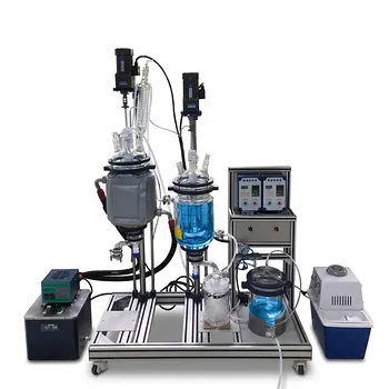
Looking to bridge the gap between chemical engineering theory and physical process operations? LABPARK provides state-of-the-art Educational and Vocational Unit Operations Pilot Plants in chemical engineering, bioprocess & biotech, and environmental & water treatment.

Designed specifically for universities, research institutes, and enterprises, our high-precision pilot plants feature the reliable instrumentation needed to validate thermodynamic models like the Rachford-Rice equation in real time.

Ready to elevate your engineering training and research capabilities? Contact LABPARK today to discuss your custom pilot plant requirements!