How Does Chromatography Zone Separation Work? Optimize System Design

Zone separation is the central mechanism that makes continuous counter-current chromatography a powerful purification tool. In this system, specific zones perform distinct tasks: above the feed point, desorbent strips the strongly adsorbed component to produce the extract, while below the feed, the weakly adsorbed component stays in the liquid phase as raffinate, and the remaining impurities are re‑adsorbed to regenerate the desorbent. The critical impact of the stripping and absorption coefficients is that when either approaches 1.0, separation becomes extremely difficult—demanding a much higher number of stages, which increases equipment complexity and pressure drop.

The four‑zone architecture enables a seamless loop of separation and desorbent recycling, but its practical performance hinges on the stripping coefficient in Zone I and the absorption coefficient in Zone IV. If these coefficients drift close to unity, the mass‑transfer driving force collapses, forcing you to add many more columns just to reach target purity and recovery. That dramatically raises capital cost, operational pressure, and process complexity.

Deconstructing the Separation Zones

In a continuous counter-current system, the column train is divided into functional zones that dictate how components move between the solid stationary phase and the liquid mobile phase. Although typical Simulated Moving Bed designs use four zones, the primary reference highlights two that are paramount for product purity and solvent recovery.

The Zone Above the Feed: Extract Generation (Zone I)

Here, fresh desorbent enters and washes the stationary phase, selectively stripping the component that binds most strongly. The stripped component exits as the extract product.

The effectiveness of this stripping step determines how cleanly the strong component is recovered. If it does not readily desorb, the product remains trapped, reducing yield.

The Zone Below the Feed: Raffinate Formation and Desorbent Regeneration (Zone IV)

In this zone, the weakly adsorbed component remains largely in the mobile phase and is collected as the raffinate. Simultaneously, any remaining impurities are re-adsorbed onto the stationary phase so that the regenerated desorbent can be recycled.

This dual role—product harvesting plus solvent cleanup—makes Zone IV indispensable for both economy and sustained operation.

The Critical Role of Stripping and Absorption Coefficients

Stripping and absorption coefficients are equilibrium ratios that quantify how a component partitions between the stationary phase and the mobile phase in the respective zones. They are the invisible levers that control how many separation stages are needed.

What the Stripping Coefficient Means in Practice

In Zone I, the effective stripping coefficient (often denoted as the distribution ratio) compares the concentration of the strongly adsorbed component on the solid phase to that in the liquid phase. A high coefficient means the component clings tightly, requiring many solvent washes. A coefficient close to 1.0 indicates it partitions almost equally between the two phases—you cannot easily drive it into the liquid stream.

What the Absorption Coefficient Means for Desorbent Purity

In Zone IV, the effective absorption coefficient describes how well the weakly adsorbed or impurity components stick to the solid. When this coefficient nears 1.0, the impurities show little preference for the solid phase, meaning they contaminate the recycled desorbent and ultimately degrade the separation.

The Unity Trap: Why 1.0 Is a Disaster

When either coefficient hovers around 1.0, each theoretical stage provides only a tiny compositional shift. The separation no longer “wants” to happen spontaneously. To compensate, you must string many more physical columns together to achieve the same end purity and recovery.

Understanding the Trade-offs

The jump from a favorable coefficient (e.g., 5 or higher) to one near 1.0 is not linear—it triggers a cascade of design consequences. Ignoring this reality leads to oversized, expensive plants that still underperform.

The Multiplier Effect on Column Count

A coefficient of 1.0 means zero net partitioning advantage per stage. Even a small deviation, like 1.05, still demands a massive increase in the number of stages compared to a system with a coefficient of 2 or 3. For example, a separation that required 8 columns may suddenly need 20 or more.

Pressure Drop and Operational Cost Penalty

Adding more columns directly increases the overall pressure drop across the system. Higher pressure requires larger pumps, more robust seals, and greater energy consumption. The operational cost can easily spiral beyond budget.

Complexity Pitfalls to Avoid

Underestimating pilot‑scale data: Coefficients measured in a single equilibrium experiment may differ from those in a continuous counter-current setup due to mass‑transfer limitations.
Ignoring sorbent‑desorbent pairing: A change in desorbent can shift both coefficients away from 1.0, often more economically than simply adding columns.
Disregarding temperature effects: Slight temperature adjustments can move an unfavorable coefficient into a workable range, so treat temperature as a design variable, not a fixed parameter.

How to Apply This to Your Project

Your path forward depends entirely on where your target coefficients stand and what you prioritize most. Use these guidelines to shape a robust design strategy.

If your coefficients are well above 1.5: You can focus on optimizing flow rates, column length, and cycle time rather than fighting for more stages. A compact, cost‑effective system is within reach.
If any coefficient is perilously close to 1.0: Prepare for a larger capital investment in columns and pressure‑rated equipment. Explore alternative sorbents or desorbents first to shift the equilibrium away from unity—that single change can cut stage count by half.
If you are scaling up from bench experiments: Insist on measuring the effective stripping and absorption coefficients under the exact continuous‑flow conditions you plan to use. A minor discrepancy in the lab can translate into a wholly impractical plant design.

Understanding the intimate link between zone function and these coefficients is what separates a resilient, efficient counter-current chromatographic process from a costly engineering headache.

Summary Table:

Metric / Parameter	Impact of Favorable Coefficient (> 1.5)	Impact of Coefficient Near Unity (~ 1.0)
Stage Count	Low (fewer columns required)	Extremely High (many columns needed)
Pressure Drop	Minimal / manageable	High (increases pump and seal wear)
Purity & Yield	High recovery with minimal solvent	Low purity, high risk of recycling impurities
Capital Cost	Low to moderate	High (due to system complexity)

Bring Industrial-Scale Chromatography into Your Lab

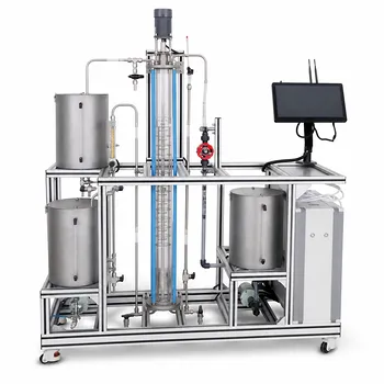
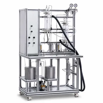
Optimizing complex separation zones requires the right hands-on training and research equipment. LABPARK provides state-of-the-art Educational and Vocational Unit Operations Pilot Plants in chemical engineering, bioprocess & biotech, and environmental & water treatment.

Designed specifically for universities, research institutes, and enterprises, our pilot plants bridge the gap between theoretical chromatography principles and real-world industrial operations.

Ready to elevate your research or training programs? Contact us today to discuss your custom pilot plant requirements!