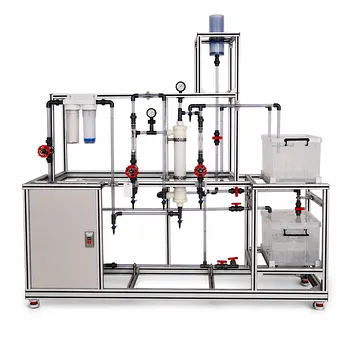
How Can Students Calculate And Optimize The Productivity Of A Batch Filtration Unit Operations Pilot Plant? (Guide)

Calculating the hourly output is just the start—the real challenge is finding the cycle time that maximizes it.** Students can calculate batch filtration productivity using the formula $Q = \frac{3600 V}{\theta + \theta_w + \theta_d}$, where $V$ is the filtrate volume per cycle and the denominator represents the total cycle time. Optimization requires running a pilot plant to experimentally measure how filtrate volume ($V$) increases with filtration time ($\theta$), and then plotting the calculated productivity ($Q$) against different $\theta$ values to find the mathematical maximum.

The core insight is that the true bottleneck for batch filtration productivity is often not the filtration step itself, but the non-productive downtime. Effective optimization shifts from a narrow focus on flow rates to a systemic analysis of the entire cycle, including cleaning and discharge, guided by experimental data from the pilot plant.

Deconstructing the Productivity Calculation

The foundation of any optimization effort is a precise, real-world calculation of the current state. The pilot plant provides the data to move beyond textbook examples.

Mapping the Total Cycle Time

The first step is to stop thinking of filtration as a single event. Students must log the complete “recipe” of the operation.

A batch filter press cycle ($T$) is the sum of three distinct phases: filtration time ($\theta$), washing time ($\theta_w$), and a critical catch-all called auxiliary operations time ($\theta_d$). This final phase includes the often-overlooked steps of cake discharge, cleaning, and reassembling the press. In a pilot plant setting, these times are measured directly, exposing how even small delays in manual cleaning can dominate the total cycle.

Calculating the Hourly Rate

Once you have the total time for a cycle and know the volume of filtrate collected ($V$), a standardized productivity metric can be calculated.

The formula $Q = \frac{3600 V}{\theta + \theta_w + \theta_d}$ converts the liters-per-cycle measurement into an hourly rate in $\text{m}^3/\text{h}$. This normalization is crucial because it allows for a direct comparison between a short cycle with a small volume and a long cycle with a large volume. It reframes the problem from simply “collecting more filtrate” to “maximizing the collection rate.”

The Experimental Path to Optimization

Theoretical equations for cake resistance are invaluable, but true optimization comes from generating a performance curve with the actual slurry and pilot-scale equipment.

Generating an Operating Curve

Optimization is a multi-variable problem that is best solved graphically using experimental data.

By running multiple cycles at a constant pressure but stopping at different filtration times ($\theta$), students record the corresponding $V$ and the fixed $\theta_d$ for each run. They then calculate $Q$ for each point. Plotting $Q$ on the y-axis against $\theta$ on the x-axis will reveal a curve that rises to a peak and then slowly declines, clearly visualizing the point of diminishing returns where a longer filtration time actually hurts the hourly rate.

Identifying the Cycle Time Sweet Spot

The experimental curve directly shows the optimal economic trade-off for a single piece of equipment.

The ascending part of the curve shows that at short times, the high volume gain from extending the run outweighs the penalty of a fixed downtime. The peak represents the optimal cycle time where hourly productivity is maximized. The descending part of the curve confirms that eventually, the filtering slows down so much that it’s more productive to stop, discharge the cake, and start a fresh, faster cycle. This teaches a counter-intuitive but vital principle: running a machine to its absolute endpoint is often unproductive.

Understanding the Trade-offs

The pursuit of raw productivity ($Q$) introduces practical conflicts. A student must recognize that maximizing the hourly rate can create downstream problems.

The Cake Depth Penalty

Higher productivity is often achieved with shorter cycles that produce thinner filter cakes. While this maximizes $Q$, it creates a trade-off in manual or automated discharge. A very thin cake can be harder to cleanly and efficiently discharge from a plate-and-frame press, potentially increasing the auxiliary time ($\theta_d$) for the next run. The pilot plant exposes this physical feedback loop that a simple theoretical model may miss.

The Unit Production Cost Blind Spot

Optimizing $Q$ in isolation ignores a higher-level economic metric: unit product cost. Continuing a run to build a thicker cake might lower the hourly filtration rate ($Q$), but if it significantly reduces the waste from product loss during discharge or minimizes the total cleaning cycles per batch campaign, it can actually lower the cost per kilogram of final product. The lab teaches that the technical optimum is not always the economic optimum.

From Unit Operation to System-Level Bottleneck

A single filter press never operates in a vacuum. Its true productivity is defined by its role in a sequence of pilot plant equipment.

Constructing the Process Gantt Chart

Integrated pilot plants allow students to map a multi-step process recipe—from a reactor to a Nutsche filter and into a dryer—onto a timeline.

By recording the occupancy time for each piece of equipment across multiple batches, students can build a Gantt chart. This visual tool immediately reveals that in overlapping, non-stop production, the overall system cycle time is dictated by the bottleneck stage—the piece of equipment with the longest processing time and the least idle time. The filter’s productivity becomes irrelevant if it’s always starved by a slower upstream reactor.

The Impact of Equipment Utilization

The analysis shifts from “how fast can I filter?” to “how long is my filter idle?”

Hands-on scheduling experiments demonstrate that adding an auxiliary unit, like a second receiving tank, can shift the process bottleneck away from the filtration step. This frees the filter to operate at its own optimal $Q$ without being the limiting factor in the overall plant’s makespan. The lesson is that system-wide productivity is a scheduling problem, not just a unit operation problem.

Making the Right Choice for Your Experiment

The optimization goal you choose will determine how you operate the pilot plant. Here’s how to align your experiment with the correct objective.

If your primary focus is maximizing the unit’s hourly rate: Run multiple cycles at constant pressure, stopping at different $\theta$ values. Plot the $Q$ vs. $\theta$ curve to experimentally find the peak productivity and accept the practical challenges of thinner cakes.
If your primary focus is minimizing unit production cost: Track all consumables, including cleaning solvents and product loss during discharge, for different cycle lengths. Calculate the total cost per kilogram of dry product to find the true economic optimum, which will likely involve a longer, slower cycle.
If your primary focus is overall plant throughput: Don’t start with the filter. Map the entire recipe on a Gantt chart to identify the system bottleneck first. Optimize the filter’s cycle time only after ensuring it is the true limiting constraint.

By moving beyond a single equation, students learn that optimization is a layered investigation into equipment physics, economic logic, and process scheduling.

Summary Table:

Optimization Parameter	Key Formula / Metric	How to Optimize in the Lab
Total Cycle Time ($T$)	$T = \theta + \theta_w + \theta_d$	Minimize non-productive downtime (cleaning, discharge $\theta_d$).
Hourly Productivity ($Q$)	$Q = \frac{3600 V}{\theta + \theta_w + \theta_d}$	Plot $Q$ vs. filtration time ($\theta$) to find the peak (diminishing returns).
System Throughput	Gantt Chart / Bottleneck Analysis	Align filter cycles with upstream/downstream equipment occupancy times.

Bring Hands-On Process Optimization to Your Lab

Teaching batch filtration and process optimization requires robust, industrial-grade equipment. LABPARK provides premium Educational and Vocational Unit Operations Pilot Plants in chemical engineering, bioprocess & biotech, and environmental & water treatment.

Designed specifically for universities, research institutes, and enterprises, our pilot plants enable students to bridge the gap between theoretical formulas and real-world industrial operations.

Ready to upgrade your engineering curriculum? Contact LABPARK today to explore our pilot plant solutions!