How To Model Battery Plate Polarization & Potential? A 1D/2D Coupling Guide For Pilot Plant Research.

The immediate answer: Researchers couple a one-dimensional micromodel of the cell element with a two-dimensional model of the electrode grid, then curve‑fit the polarization parameters—open‑circuit potential (U) and cell element conductance (Y)—as functions of depth of discharge and local current density. By applying Kirchhoff’s law to these fitted parameters, they solve for the local potential distribution across the entire plate, revealing how current evolves from strongly non‑uniform to nearly uniform as discharge proceeds.

Modeling the local potential distribution in a battery plate is not a single‑scale task; it requires linking the microscopic electrochemistry inside the porous electrode to the macroscopic current flow in the grid. When this is combined with the kind of cyclic charge‑discharge data that a chemical engineering pilot plant can generate, the model becomes a powerful tool for interpreting material utilization and degradation.

Deconstructing the Battery Plate Problem

Why a Single‑Scale Model Falls Short

A battery plate is a multi‑scale system. At the pore level, reactions occur locally, influenced by electrolyte concentration, active material state, and transport limitations. At the plate level, the metallic grid distributes current, but its resistance causes voltage drops that vary across the face. A model that ignores one scale cannot capture the true local overpotentials that drive non‑uniform consumption of active material.

The Engineer’s Solution: Coupled Micro‑ and Macro‑Models

To bridge this gap, researchers split the problem. A one‑dimensional (1D) micromodel describes the through‑thickness electrochemistry of a single cell element—the sandwich of positive active material, separator, and negative active material. This micromodel yields the two fundamental polarization parameters:

Open‑circuit potential (U) – the equilibrium voltage as a function of the state of charge.
Cell element conductance (Y) – the local ease with which charge transfers across the electrode, reflecting both kinetic and ohmic resistances.

These parameters then feed into a two‑dimensional (2D) grid model that represents the extended current collector and the active material coating. By solving for current flow in this distributed network, the model reveals the potential field across the entire plate.

Parameterizing Polarization with Pilot Plant Experiments

Extracting U and Y from Charge‑Discharge Data

In a chemical engineering pilot plant, trainees and researchers run full charge‑discharge cycles under controlled constant‑current or constant‑voltage regimes. The voltage–capacity curves from these cycles are the raw input for curve‑fitting. Because U and the apparent conductance both depend on depth of discharge (DoD), data from a single cycle can be used to map out the equilibrium potential and the total cell resistance as the electrode is progressively discharged.

The Critical Role of Depth of Discharge and Local Current Density

The polarization parameters are not constants. U shifts as the active material’s composition changes with DoD. Similarly, Y varies because the local current density influences concentration overpotentials and ohmic drops in the pore electrolyte. By treating U and Y as functions of both DoD and the local reaction current, researchers can accurately replicate the feedback loop: as more current flows in a region, its state of charge changes faster, altering U and Y and thereby redirecting current to other regions.

Solving the Potential Field and Current Distribution

Applying Kirchhoff’s Law to a Distributed Network

Once U and Y are parameterized, the 2D grid model becomes a network of nodes connected by the grid’s metallic resistance. At each node, the local current entering the active material must satisfy Kirchhoff’s current law—what flows in from the grid equals the electrochemical reaction current, which is determined by the local U and Y. Solving this large set of algebraic equations yields the local potential distribution and the corresponding current density map across the plate face.

The Evolution from Non‑Uniform to Uniform Current

At the start of discharge, the grid ohmic drop is highest near the current tab, so current density is strongly non‑uniform—edges and far corners receive less current. However, because the electrochemical resistance and apparent open‑circuit potential depend directly on the state of charge, the ohmic penalty is gradually compensated. Regions that react faster deplete first, causing their U to shift unfavorably and their Y to increase, which naturally forces current toward previously under‑utilized areas. As discharge proceeds, the distribution becomes markedly more uniform.

Connecting the Model to Pilot Plant Observations

Explaining Material Utilization Efficiency

In pilot plant training, students often measure that only 70% to 80% of the theoretical capacity is accessible—a figure that drops with cycling. The coupled model provides a root‑cause explanation. Early non‑uniform current can isolate microscopic active material particles (reducing electronic contact), block pores with reaction products, or dissolve soluble reactants. These degradation pathways manifest in the model as a local reduction in Y or a hysteresis in U that extends beyond the simple DoD dependence.

Diagnosing Degradation with Polarization Trends

By comparing model predictions with experimental voltage‑cutoff curves and capacity fade data, researchers can attribute loss mechanisms to specific model parameters. For example, a steady decline in the average cell element conductance Y points to pore blockage or increased solid‑electrolyte interphase resistance, while a shift in the U–DoD curve suggests active material phase changes or loss of accessible redox centers. This diagnostic loop is exactly what a pilot plant enables: iterative cycling under different protocols yields the degradation fingerprints needed to refine the polarization functions.

Practical Trade‑offs in Modeling and Experimentation

No modeling approach is free of compromises. The following trade‑offs must be managed when applying this method in a pilot plant setting.

Model fidelity vs. computational cost: A fully coupled 3D micro‑macro model with detailed pore‑level kinetics is computationally heavy. The 1D+2D framework reduces complexity but assumes through‑thickness uniformity in the grid plane. For thick plates or high‑rate discharges, this assumption may weaken.

Data availability vs. parameter certainty: Curve‑fitting U and Y requires high‑quality voltage–capacity traces at multiple rates and depths. If pilot plant data is sparse or noisy, the fitted functions may over‑smooth real non‑linearities, masking early signs of uneven utilization.

Generality vs. system specificity: The parameterization is inherently tied to a specific cell chemistry and plate design. Extrapolating U and Y from one pilot‑plant configuration to another requires careful accounting for changes in active material loading, grid geometry, or electrolyte composition.

Making the Right Choice for Your Pilot Plant Studies

Your experimental objectives will dictate how deeply you need to embed this coupled modeling approach.

If your primary focus is training and visualizing non‑uniformity: Use the 1D+2D framework to show how grid resistance creates a current distribution map. Even a simplified parameterization from a single constant‑current discharge can vividly demonstrate the self‑equalizing effect.
If your primary focus is optimizing plate design for higher material utilization: Invest in multiple constant‑current and constant‑voltage cycles. Fit U and Y over a wide DoD range and validate the model’s ability to predict the 70–80% utilization limit. Then use it to test virtual changes in grid tab placement or active material formulation.
If your primary focus is lifetime prediction and degradation analysis: Combine the model with accelerated cycling data. Track how U(Y) evolves cycle by cycle and link parameter drifts to physical degradation mechanisms like pore blockage or reactant dissolution. This turns your pilot plant from a testing bench into a diagnostic instrument.

When you embed the coupled polarization model into your pilot plant workflow, you transform raw voltage‑time curves into a window onto the hidden current landscape of a battery plate—giving you the power to design, diagnose, and educate with far greater precision.

Summary Table:

Modeling Element	Description	Role in Battery Plate Analysis
1D Micromodel	Through-thickness electrochemistry of cell element	Determines local polarization parameters ($U$ and $Y$)
2D Grid Model	Distributed network of the current collector grid	Solves Kirchhoff's laws for local potential distribution
Open-Circuit Potential ($U$)	Equilibrium voltage as a function of Depth of Discharge	Captures thermodynamic changes during discharge
Conductance ($Y$)	Ease of charge transfer across the electrode	Captures kinetic and ohmic resistance variations

Scale Up Your Chemical Engineering Research with LABPARK

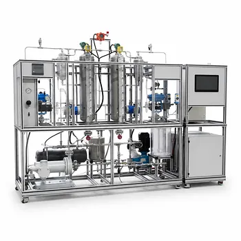
Are you looking to bridge the gap between electrochemical theory and practical industrial application? LABPARK provides premium Educational and Vocational Unit Operations Pilot Plants in chemical engineering, bioprocess & biotech, and environmental & water treatment designed specifically for universities, research institutes, and enterprises.

Our pilot plants empower researchers and students to generate the high-fidelity cyclic charge-discharge data required for advanced polarization modeling, degradation diagnostics, and system optimization.

Contact us today to explore our customizable pilot plant solutions and elevate your laboratory's training and research capabilities!