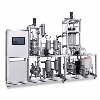
How To Determine Lle Theoretical Stages In A Pilot Plant? A Complete Guide

The most critical realization is that these calculations are a bridge, not a destination. Researchers and students don't just calculate a number; they use the pilot plant to validate those calculations against reality. For partially miscible systems, you plot the feed, solvent, and mixture points on a triangular phase diagram and step off stages using the operating point. For completely immiscible systems, you use a simpler X-Y diagram with an operating line or an analytical Kremser-type equation. The pilot plant then executes the process, allowing you to measure outlet concentrations and calculate the actual stage efficiency by comparing the theoretical number of stages to the physical number of stages in the unit.

A pilot plant’s true purpose in this context is not to be a calculator. It is to be a verifier of models. Your core task is to use the plant’s empirical concentration data to determine "stage efficiency"—the quantifiable gap between an idealized mathematical stage and a real, physical piece of equipment.

The Theoretical Foundation: Choosing Your Method Based on Miscibility

The calculation strategy hinges entirely on how the liquid phases behave together.

For Completely Immiscible Systems: The Simplified X-Y Method

When the carrier and solvent don't dissolve in each other, the calculations become straightforward. This is common in aqueous-organic extractions.

You create a rectangular coordinate system. You plot the equilibrium distribution curve, which relates solute concentration in the extract to its concentration in the raffinate. You then draw an operating line derived from a simple mass balance around a section of the column. This line has a slope determined by the flow rates of the two carrier streams.

You step off the stages by constructing a staircase between the equilibrium curve and the operating line, starting from the known feed point. Each step represents one theoretical stage.

For Partially Miscible Systems: The Triangular Phase Diagram

When the solvent and carrier have significant mutual solubility, the analysis moves to a ternary plot. This is a more visually complex but powerful tool.

The procedure is a systematic four-step process:

Locate the Mixture Point (M): You plot the pure feed (F) and solvent (S) on the diagram. The M point lies on the line connecting them. Its exact position is determined by the solvent-to-feed (S/F) ratio.
Determine End Compositions: The tie line that passes through M, if you're lucky, or is interpolated, intersects the solubility curve to give you the theoretical extract (E) and raffinate (R) phases leaving the first ideal stage.
Find the Operating Point (Δ): This is the real key. You draw lines through the final raffinate composition (R_final) and the solvent (S), and through the final extract (E_final) and the feed (F). The intersection of these two lines is the net flow operating point, Δ.
Step Off the Stages: Starting from the raffinate composition (R1) of the first stage, you draw a line to Δ. Where this line intersects the extract side of the solubility curve is the extract (E2) from the next stage. You then follow the tie line to find R2, and repeat until you pass R_final.

From Theory to Reality: The Crucial Role of the Pilot Plant

The physical pilot plant serves one primary function for this analysis: to expose the inefficiency of real-world mass transfer.

The Core Objective: Determining Stage Efficiency

A theoretical stage represents an equilibrium condition that physical equipment almost never achieves. A real stage can only approach this ideal state. The pilot plant quantifies this gap.

Stage efficiency is the metric that bridges theory and reality. You calculate the theoretical stages needed for a desired separation using the methods above. Then, you run the process in a pilot plant with a known number of physical stages. The efficiency is the ratio: theoretical stages divided by actual physical stages.

The Experimental Process: Measuring and Comparing

This is where the research or educational value crystallizes. You operate the pilot plant—whether it’s a mixer-settler, a pulsed column, or a packed tower—at steady state.

You then take liquid samples from the feed, solvent, final extract, and final raffinate ports. By measuring solute concentrations in these streams, you can back-calculate the operating line and equilibrium relationship the process actually followed. Plotting this empirical data against the theoretical model you built earlier directly reveals the number of theoretical stages the pilot plant effectively provided.

Factors That Influence Real-World Performance

The mismatch between a theoretical and a real stage isn't random. It’s a direct consequence of fluid properties and equipment design, which the pilot plant helps you study.

Interfacial Tension: It must be moderate. High tension prevents good dispersion, while low tension can create stable emulsions that hinder phase separation. Both outcomes destroy stage efficiency.
Density Difference: A large density difference between the extract and raffinate phases is a prime driver. It accelerates gravity-driven settling, a bottleneck in many liquid-liquid processes.
Viscosity: High viscosity in either phase slows down solute diffusion, directly reducing the mass transfer rate achievable in a single stage.

Understanding the Trade-offs and Limitations

No single method or piece of equipment is without significant drawbacks. Recognizing these is essential for valid research.

The Limits of Graphical Methods

Graphical techniques, while pedagogically excellent, are inherently time-consuming and prone to human error. Constructions on a triangular diagram or X-Y plot rely on accurate tie-line data, which can be scarce for new systems.

The Assumptions Behind Analytical Equations

The Kremser-type equation is elegant but restrictive. It assumes a constant distribution coefficient (K) and constant carrier-to-solvent flow ratios across all stages. For highly non-ideal or concentrated solutions, this assumption crumbles, making the equation's output an approximation at best.

Equipment Realities and Scale-Up Challenges

Choosing the wrong pilot-scale equipment can obscure your results entirely. For instance, a system needing only 3 easy stages will be poorly characterized in a complex rotating disc column designed for 15 stages. Conversely, a difficult separation requiring 10 stages cannot be resolved in a simple spray tower with only 3 effective stages. The equipment’s inherent efficiency and throughput capacity must match the separation’s theoretical demand and the fluid’s physical properties.

Making the Right Choice for Your Research or Educational Goal

Your specific objective should dictate how you integrate pilot plant work with theoretical stage calculations.

If your primary focus is deep conceptual understanding: Start with the graphical methods—triangular diagrams for complex systems, X-Y plots for simple ones. Use the pilot plant purely as a visual, tactile demonstration to reinforce the mass-balance principles.
If your primary focus is rapid process design and iteration: Use the analytical Kremser-type method for an initial estimate, then run a targeted experiment on the pilot plant to measure the actual efficiency of your chosen equipment and refine your design factor.
If your primary focus is scale-up and industrial feasibility: Conduct a series of pilot plant experiments to map how stage efficiency changes with varying flow rates, phase ratios, and agitator speeds. This empirical map is the cornerstone of sound scale-up.

Bridging the gap between the idealized stage and the metal, glass, and gaskets of a pilot plant is the very essence of chemical engineering practice.

Summary Table:

System Type	Calculation Method	Key Tool / Diagram	Pilot Plant Role
Completely Immiscible	Simplified X-Y Method	Rectangular coordinate (equilibrium & operating lines)	Measure outlet conc. & calculate stage efficiency
Partially Miscible	Triangular Phase Diagram	Ternary plot (solubility curve, tie lines, operating point)	Validate mathematical models against physical stages

Optimize Your Chemical Engineering Lab with LABPARK

Are you looking to bridge the gap between theoretical calculations and real-world process validation? LABPARK provides state-of-the-art Educational and Vocational Unit Operations Pilot Plants in chemical engineering, bioprocess & biotech, and environmental & water treatment. Designed specifically for universities, research institutes, and enterprises, our pilot plants enable hands-on learning, precise model verification, and reliable scale-up studies.

Contact our team today to find the perfect pilot plant for your institution!