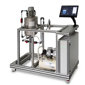
How Can Fluid Mechanics Unit Operation Training Units Visually Demonstrate Flow? See Laminar-To-Turbulent Transition In Action

A fluid mechanics training unit can make the laminar-to-turbulent transition visible by injecting a thin colored-fluid filament into a transparent pipe while gradually increasing the flow rate. At low velocity, the dye remains a narrow, straight line parallel to the pipe axis, indicating laminar flow. As velocity increases, the filament develops irregular transverse motions and eventually disperses across the pipe, revealing transitional and turbulent flow.

The visual transition is governed primarily by the Reynolds number, which compares inertial forces with viscous forces. In a circular pipe, laminar flow is typically observed below (Re \approx 2300), while fully turbulent behavior generally develops above approximately (Re \approx 4000); the range between these values is transitional and sensitive to disturbances.

How the Training Unit Shows the Transition

The Transparent Test Section

A typical Reynolds-flow demonstration unit uses a transparent glass or plastic pipe, a water reservoir, a pump or gravity-fed supply, a flow-control valve, and a flow-measurement device.

The transparent section allows students to observe the dye and compare the visible flow pattern with measured velocity, pipe diameter, fluid properties, and pressure drop.

The Dye-Injection System

A needle introduces a thin stream of colored liquid into the center of the flowing fluid. The injection must be steady and sufficiently fine so that the dye reveals the surrounding flow rather than creating a large disturbance of its own.

The apparatus is usually operated after the upstream flow has been allowed to settle, reducing unwanted inlet disturbances that could obscure the transition.

The Laminar Pattern

At low flow rates, the dye forms a stable filament that moves downstream without significant spreading across the pipe. This demonstrates that the fluid is moving in relatively orderly layers with limited transverse exchange.

For fully developed laminar flow in a circular pipe, the velocity profile is parabolic: velocity is highest at the center and falls to zero at the wall because of the no-slip condition.

The Transitional Pattern

As the flow rate increases, the dye filament may begin to waver, oscillate, or break into intermittent disturbances. This is the transitional regime, where laminar and turbulent characteristics coexist.

The transition does not always appear as an instantaneous switch. The observed threshold depends on the smoothness of the pipe, the quality of the inlet flow, vibration, fittings, and the magnitude of disturbances entering the system.

The Turbulent Pattern

At higher flow rates, irregular transverse motions cause the dye to spread rapidly across the pipe cross-section. The filament loses its coherent shape and becomes a visibly mixed region.

These motions reflect fluctuating velocity components and eddies that transport momentum, fluid, heat, and dissolved species across the main flow direction.

What Physical Principles Govern the Transition?

Reynolds Number

The principal governing parameter is the Reynolds number:

[ Re = \frac{\rho u_m D}{\mu} ]

or, using kinematic viscosity,

[ Re = \frac{u_m D}{\nu} ]

where (\rho) is fluid density, (u_m) is mean velocity, (D) is pipe diameter, (\mu) is dynamic viscosity, and (\nu) is kinematic viscosity.

A high Reynolds number means that inertial effects are large relative to viscous effects. A low Reynolds number means that viscosity is more effective at damping disturbances and preserving orderly motion.

Competition Between Inertia and Viscosity

In laminar flow, viscous forces suppress velocity fluctuations and keep neighboring fluid layers moving in an organized manner. A dye filament therefore remains narrow because there is little bulk transport perpendicular to the pipe axis.

As inertia becomes more influential, disturbances can grow rather than being rapidly damped. The resulting velocity fluctuations stretch, fold, and disperse the dye.

Instability and Disturbance Amplification

Pipe-flow transition is affected by the disturbances present in the system. Pump pulsation, valves, bends, surface roughness, vibration, and an uneven inlet profile can all promote earlier transition.

The classical critical Reynolds number is therefore a practical reference rather than an immutable physical constant. In a carefully controlled system, laminar flow can persist above the usual lower threshold, while strong disturbances can produce turbulent behavior at lower values.

Velocity-Profile Changes

Laminar flow has a strongly nonuniform, parabolic velocity profile. Turbulent mixing transports momentum toward and away from the wall, producing a flatter central velocity profile with a steep velocity gradient near the wall.

Even in turbulent pipe flow, a thin near-wall viscous sublayer remains important. The flow is therefore not turbulent in exactly the same way at every location in the pipe.

Pressure-Drop Behavior

For fully developed laminar flow, the Hagen-Poiseuille relationship gives:

[ \Delta p \propto u_m ]

for fixed fluid properties, pipe diameter, and length. Pressure drop increases directly with mean velocity.

In turbulent flow, pressure loss is commonly correlated through a friction factor, and under many practical conditions the pressure drop scales approximately with (u_m^2). The exact relationship depends on Reynolds number, pipe roughness, and the applicable friction-factor correlation.

Why the Demonstration Matters in Unit Operations

Mixing and Mass Transfer

Laminar flow produces limited transverse mixing, so species may remain stratified as they move through the pipe. Turbulent flow enhances mixing by creating fluctuating motion and increased momentum exchange.

This distinction affects residence-time behavior, blending, chemical reaction, dissolution, and mass-transfer performance in process equipment.

Heat Transfer

Turbulent motion continually transports fluid from the bulk toward regions near the wall. This usually reduces the thickness of the thermal boundary layer and increases convective heat-transfer rates compared with laminar flow at comparable conditions.

The transition experiment therefore connects a visible dye pattern with practical heat-exchanger and reactor performance.

Equipment Design and Scale-Up

The same flow rate can produce different regimes in pipes of different diameters or with fluids of different viscosities. Engineers must therefore compare Reynolds numbers rather than relying on volumetric flow rate alone.

A pilot unit allows students to connect flow regime, pressure loss, pump demand, mixing quality, and transport coefficients before applying those relationships to larger systems.

Understanding the Trade-Offs

The Dye Pattern Is Qualitative

A straight filament strongly suggests orderly flow, and rapid dispersion is consistent with turbulence, but dye visualization alone does not measure every turbulent fluctuation. Dye diffusion, injection conditions, optical resolution, and observation distance also affect the appearance.

For quantitative work, the visual result should be combined with measured flow rate, fluid temperature, pipe diameter, and pressure drop.

The Transition Is Not a Single Universal Point

The values (Re \approx 2300) and (Re \approx 4000) are useful engineering guidelines for internal flow in smooth circular pipes. The transitional range can shift or become less distinct when the inlet is disturbed, the pipe is rough, or fittings are located near the observation point.

A training unit should therefore present the critical Reynolds number as a range and experimental indicator, not as an exact boundary that applies to every installation.

Turbulence Does Not Mean Uniform Mixing Everywhere

Turbulent flow enhances cross-sectional transport, but near-wall regions still contain strong velocity and viscosity effects. Complete mixing may also require sufficient pipe length, and a dye may not appear uniform immediately after the transition.

This is important when translating a visual demonstration into a design assumption for a real process line.

Excessive Flow Can Distort the Demonstration

A high pump setting, unstable valve position, or poorly aligned injector can create disturbances unrelated to the natural pipe-flow transition. The unit should use gradual flow adjustment and a stable dye feed so that the observed changes are attributable primarily to the changing Reynolds number.

How to Apply This to Your Project

A reliable demonstration combines visual observation with calculated Reynolds number and, where available, pressure-drop measurements.

If your primary focus is visual understanding: Use a transparent, straight test section with a fine central dye filament and increase velocity gradually while recording the stable, wavering, and dispersed patterns.
If your primary focus is quantitative analysis: Measure flow rate, pipe diameter, temperature, density, and viscosity, then calculate (Re) and compare the observed regime with pressure-drop data.
If your primary focus is process design: Use the observed regime to assess how velocity affects mixing, heat transfer, mass transfer, wall shear, and pumping requirements.
If your primary focus is transition research: Control inlet disturbances, fittings, pipe roughness, and vibration while using flow meters, differential-pressure sensors, and visualization to study why the transition threshold changes.

By combining dye visualization with Reynolds-number calculations and pressure measurements, a training unit turns an abstract flow-regime criterion into an observable and useful engineering principle.

Summary Table:

Key aspect	Laminar flow	Transitional flow	Turbulent flow
Typical Reynolds number	Below 2300	About 2300-4000	Above 4000
Dye appearance	Thin, straight filament	Wavering or intermittent filament	Rapidly dispersed and mixed dye
Dominant forces	Viscous forces	Competing inertia and viscosity	Inertial forces
Velocity profile	Parabolic	Developing fluctuations	Flatter core with steep near-wall gradient
Pressure-drop trend	Approximately proportional to velocity	Sensitive to disturbances	Often approximately proportional to velocity squared
Engineering relevance	Limited mixing and lower transport rates	Sensitive operating regime	Enhanced mixing, heat transfer, and mass transfer
Key influences	Fluid properties, diameter, and velocity	Inlet conditions, fittings, vibration, and roughness	Reynolds number, roughness, and flow development

See fluid-flow principles in action with LABPARK Educational and Vocational Unit Operations Pilot Plants. Our fluid mechanics training units help universities, research institutes, and enterprises demonstrate laminar, transitional, and turbulent pipe flow through transparent test sections, controlled dye injection, flow measurement, and pressure-drop analysis. Connect Reynolds number calculations with practical lessons in mixing, heat transfer, mass transfer, pump demand, and process scale-up. Contact LABPARK to discuss a pilot plant configured for your teaching, research, or industrial training requirements.